Page 237 - Numerical Analysis Using MATLAB and Excel

Chapter 6 Fourier, Taylor, and Maclaurin Series

– 2π – π 0 π 2π 3π
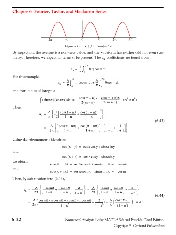
Figure 6.18. ft() for Example 6.6

By inspection, the average is a non−zero value, and the waveform has neither odd nor even sym-
metry. Therefore, we expect all terms to be present. The a n coefficients are found from

1 2π
d
a = --- ∫ ft()cos nt t
π
n
0
For this example,
A π A 2π
d
d
a = ---- ∫ sin tcos nt t + ---- ∫ 0cos nt t
π
n
0 π π
and from tables of integrals
(
)
cos
m +
)
mn x
( cos
–
∫ ( sin mx cos nx x = – ------------------------------ – ------------------------------- m ≠( n n x 2 n ) 2
(
)
)
d
(
)
(
)
–
2m +
2m n
Then,
A ⎧ 1 cos ( 1 – n t ( cos 1 + n t π ⎫
)
)
a = ---- – -- --------------------------- + ---------------------------- ⎬
-
⎨
n
π
1 +
n
–
1n
2
⎩
⎭
0
(6.43)
A ⎧ cos ( π – nπ ) cos ( π + nπ ) 1 1 ⎫
= – ------ ⎨ ----------------------------- + ------------------------------ – ------------ + ------------ ⎬
2π ⎩ 1 – n 1 + n 1n n + 1 ⎭
–
Using the trigonometric identities
)
–
( cos xy = cos xcos + sin xsiny
y
and
)
( cos x + y = cos xcos y – sin xsin y
we obtain
)
cos ( π – nπ = cos πcos nπ + sin πsin nπ = – cos nπ
and
)
cos ( π + nπ = cos πcos nπ – sin πsin nπ = – cos nπ
Then, by substitution into (6.43),
A ⎧ – cos nπ – cos nπ 2 ⎫ A ⎧ cos nπ cos nπ 2 ⎫
a = – ------ ⎨ 2π ------------------ + ------------------ – -------------- ⎬ 2 = ------ ⎨ --------------- + --------------- + -------------- ⎬ 2
n
2π
1 –
–
1 +
1 +
n
n
1n
n
1 –
⎩
n ⎭
1 –
⎩
n ⎭
(6.44)
A cos nπ + ncos nπ + cos nπ – ncos nπ 2 ⎞ A cos nπ + 1
⎛
⎛
= ------ --------------------------------------------------------------------------------------- + -------------- = ---- ------------------------- ⎞ n ≠ 1
2π ⎝ 1 – n 2 1n 2⎠ π ⎝ ( 1 – n ) 2 ⎠
–
6−20 Numerical Analysis Using MATLAB® and Excel®, Third Edition
Copyright © Orchard Publications