Page 239 - Numerical Analysis Using MATLAB and Excel

Chapter 6 Fourier, Taylor, and Maclaurin Series

and from tables of integrals,

(
m +
n x
(
)
sin
mn x
–
sin
∫ ( sin mx sin nx x = ----------------------------- – ------------------------------ m ≠( n ) ) 2 n ) 2
)
)
(
d
(
2m +
)
(
2m n
–
Therefore,
A 1⎧ ( sin 1n t ( sin 1 + n t π ⎫
)
)
–
b = ---- -- - ⎩ -------------------------- – --------------------------- 0 ⎬ ⎭
⋅ ⎨
n
π 2
n
n
1 +
1 –
A sin ( 1n π – ) ( sin 1 + n π )
= ------ ---------------------------- – ---------------------------- – 0 + 0 0 n ≠ 1 )
(=
2π 1 – n 1 + n
that is, all the b n coefficients, except b 1 , are zero.
We will find b 1 by direct substitution into (6.14) for n = 1 . Thus,
A π 2 A t sin 2t π A π sin 2π A
)
b = ---- ∫ ( sin t d = ---- -- – ------------ = ---- --- – -------------- = ---- (6.52)
t
-
1
π
0 π 2 4 0 π 2 4 2
Combining (6.45) and (6.47) through (6.52), we find that the trigonometric Fourier series for the
half−wave rectification waveform with no symmetry is
cos
8t
4t
cos
ft() = A A t A cos 2t ------------- + cos 6t ------------- + … (6.53)
---- sin –
------------- +
---- ------------- +
---- +
π 2 π 3 15 35 63
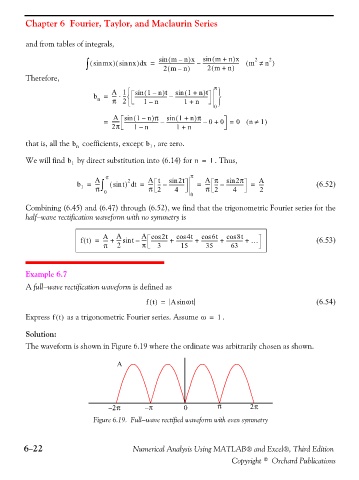
Example 6.7
A full−wave rectification waveform is defined as
ft() = Asin ωt (6.54)
Express ft() as a trigonometric Fourier series. Assume ω = . 1
Solution:
The waveform is shown in Figure 6.19 where the ordinate was arbitrarily chosen as shown.
A
1
0. 9
0. 8
0. 7
0. 6
0. 5
0. 4
0. 3
0. 2
0. 1
– 2π 2 – π 4 6 0 8 π 10 12 2π
0
0
Figure 6.19. Full−wave rectified waveform with even symmetry
6−22 Numerical Analysis Using MATLAB® and Excel®, Third Edition
Copyright © Orchard Publications