Page 245 - Numerical Analysis Using MATLAB and Excel

Chapter 6 Fourier, Taylor, and Maclaurin Series

⁄
⁄
1
1
3
–
–
---
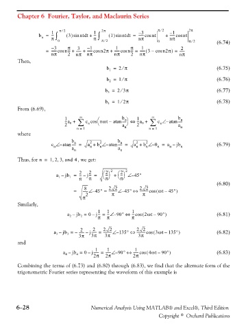
b = --- ∫ π 2 3 ()sin nt t +d 1 ∫ 2π 1 ()sin nt t = ------ cos nt π 2 + ------ cos nt 2π
d
π
n
⁄
⁄
0 π π 2 nπ 0 nπ π 2 (6.74)
– 3 π 3 – 1 1 π 1 2
)
= ------ cos n--- + ------ + ------ cos n2π + ------ cos n--- = ------ 3 –( cos n2π = ------
nπ 2 nπ nπ nπ 2 nπ nπ
Then,
⁄
b = 2 π (6.75)
1
⁄
b = 1 π (6.76)
2
⁄
b = 23π (6.77)
3
⁄
b = 12π (6.78)
4
From (6.69),
1 ∞ ⎛ b n⎞ 1 ∞ b n
-
--a + c cos ⎝ ∑ nωt – atan ----- ⇔ ---a + ∑ c ∠ – atan -----
2 0 n a ⎠ 2 0 n a
n = 1 n n = 1 n
where
b b
2
2
2
2
n
n
c ∠ – atan ----- = a + b ∠ – atan ----- = a + b ∠ – θ = a – jb n (6.79)
n
n
n
n
n
n
n
a
a
n
n
,,,
Thus, for n = 1 2 3 and 4 , we get:
2
2
2 2 ⎛⎞ 2 ⎛⎞ 2
a – jb = --- – j--- = --- + --- ∠ – 45°
1
π
1
π
π π ⎝⎠ ⎝⎠
(6.80)
8
---------- –∠
∠
= ------ – 45° = 22 45° ⇔ 22 ( ωt – 45° )
---------- cos
π 2 π π
Similarly,
1 1 1
a – jb = 0j--- = --- –∠ 90° ⇔ --- cos ( 2ωt – 90° ) (6.81)
–
π
2
2
π
π
2 2 22 22
a – jb = – ------ – j------ = ---------- –∠ 135° ---------- cos (⇔ 3ωt – 135° ) (6.82)
3
3
3π 3π 3π 3π
and
1 1 1
a – jb = 0j------ = ------ –∠ 90° ⇔ ------ cos ( 4ωt – 90° ) (6.83)
–
2π
2π
4
4
2π
Combining the terms of (6.73) and (6.80) through (6.83), we find that the alternate form of the
trigonometric Fourier series representing the waveform of this example is
6−28 Numerical Analysis Using MATLAB® and Excel®, Third Edition
Copyright © Orchard Publications