Page 250 - Numerical Analysis Using MATLAB and Excel

Line Spectra

as expected.

For n = odd , e – jnπ = – 1 . Therefore,

2A
C ------------ e ( = A – jnπ – 1 ) 2 ------------ –( = A 1 – 1 ) 2 = ------------ –( A 2 ) 2 = -------- (6.104)
n = n odd 2jπn 2jπn 2jπn jπn
Using (6.92), that is,

ft() = … + C e – j2ωt + C e – jωt + C + C e jωt + C e j2ωt + …
–
2
2
1
0
–
1
we obtain the exponential Fourier series for the square waveform with odd symmetry as
2A ⎛ 1 – j3ωt – jωt jωt 1 j3ωt ⎞ 2A 1 jnωt
-
-
-
ft() = ------- … – --e – e + e + --e = ------- ∑ --e (6.105)
jπ ⎝ 3 3 ⎠ jπ n
n = odd
The minus (−) sign of the first two terms within the parentheses results from the fact that
⁄
⁄
C – n = C ∗ . For instance, since C = 2A j3π , it follows that C – 3 = C ∗ = – 2A j3π . We
3
3
n
observe that ft() is purely imaginary, as expected, since the waveform is an odd function.
To prove that (6.105) and (6.22) are the same, we group the two terms inside the parentheses of
(6.105) for which n = 1 ; this will produce the fundamental frequency sin ωt . Then, we group
the two terms for which n = 3 , and this will produce the third harmonic sin 3ωt , and so on.

6.7 Line Spectra

When the Fourier series are known, it is useful to plot the amplitudes of the harmonics on a fre-
quency scale that shows the first (fundamental frequency) harmonic, and the higher harmonics
times the amplitude of the fundamental. Such a plot is known as line spectrum and shows the
*
spectral lines that would be displayed by a spectrum analyzer .
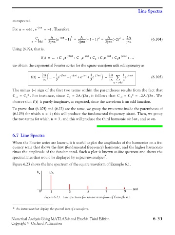
Figure 6.23 shows the line spectrum of the square waveform of Example 6.1.

b n 4/π

nωt
0 1 3 5 7 9
Figure 6.23. Line spectrum for square waveform of Example 6.1

* An instrument that displays the spectral lines of a waveform.

Numerical Analysis Using MATLAB® and Excel®, Third Edition 6−33
Copyright © Orchard Publications