Page 255 - Numerical Analysis Using MATLAB and Excel

Chapter 6 Fourier, Taylor, and Maclaurin Series

ysin3x 0.000 0.131 0.259 0.383 0.500 0.609 0.707 0.793 0.866 0.924 0.966 0.991 1.000 0.991 0.966 0.924 0.866 0.793 0.707 0.609 0.500

sin3x 0.000 0.131 0.259 0.383 0.500 0.609 0.707 0.793 0.866 0.924 0.966 0.991 1.000 0.991 0.966 0.924 0.866 0.793 0.707 0.609 0.500

ycos3x 0.000 0.991 0.966 0.924 0.866 0.793 0.707 0.609 0.500 0.383 0.259 0.131 0.000 -0.131 -0.259 -0.383 -0.500 -0.609 -0.707 -0.793 -0.866

cos3x ysin2x 1.000 0.000 0.991 0.087 0.966 0.174 0.924 0.259 0.866 0.342 0.793 0.423 0.707 0.500 0.609 0.574 0.500 0.643 0.383 0.707 0.259 0.766 0.131 0.819 0.000 0.866 -0.131 0.906 -0.259 0.940 -0.383 0.966 -0.500 0.985 -0.609 0.996 -0.707 1.000 -0.793 0.996 -0.866 0.985
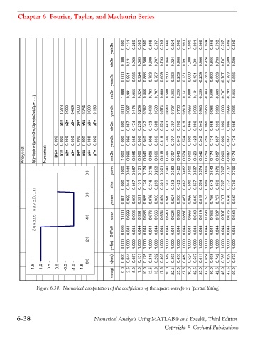
f(t)=4(sinwt/p+sin3wt/3p+sin5wt/5p+ ….) 0.000 b1= 0.000 0.000 b2= b3= 0.000 b4= 0.000 b5= 0.000 0.000 b6= b7= 0.000 sin2x 0.000 0.000 0.087 0.996 0.174 0.985 0.259 0.966 0.342 0.940 0.423 0.906 0.500 0.866 0.574 0.819 0.643 0.766 0.707 0.707 0.766 0.643 0.819 0.574 0.866 0.500 0.906 0.423 0.940 0.342 0.966 0.259 0.985 0.174 0.996 0.087 1.000 0.000 0.996 0.985
0.254
0.000
0.000
0.180
1.273
0.000
0.424

Analytical: Numerical: DC= a1= a2= a3= a4= a5= a6= a7= ycox2x cos2x 1.000 0.996 0.985 0.966 0.940 0.906 0.866 0.819 0.766 0.707 0.643 0.574 0.500 0.423 0.342 0.259 0.174 0.087 0.000 -0.087 -0.087 -0.174 -0.174

8.0 ysinx 0.000 0.044 0.087 0.131 0.174 0.216 0.259 0.301 0.342 0.383 0.423 0.462 0.500 0.537 0.574 0.609 0.643 0.676 0.707 0.737 0.766

sinx 0.000 0.044 0.087 0.131 0.174 0.216 0.259 0.301 0.342 0.383 0.423 0.462 0.500 0.537 0.574 0.609 0.643 0.676 0.707 0.737 0.766
Square waveform Average= 4.0 ycosx cosx 0.000 1.000 0.999 0.999 0.996 0.996 0.991 0.991 0.985 0.985 0.976 0.976 0.966 0.966 0.954 0.954 0.940 0.940 0.924 0.924 0.906 0.906 0.887 0.887 0.866 0.866 0.843 0.843 0.819 0.819 0.793 0.793 0.766 0.766 0.737 0.737 0.707 0.707 0.676 0.676 0.643 0.643
6.0

2.0 0.5*a0 0.000 0.044 0.044 0.044 0.044 0.044 0.044 0.044 0.044 0.044 0.044 0.044 0.044 0.044 0.044 0.044 0.044 0.044 0.044 0.044 0.044
y=f(x) 0.000 1.000 1.000 1.000 1.000 1.000 1.000 1.000 1.000 1.000 1.000 1.000 1.000 1.000 1.000 1.000 1.000 1.000 1.000 1.000 1.000

0.0 x(rad) 0.000 0.044 0.087 0.131 0.175 0.218 0.262 0.305 0.349 0.393 0.436 0.480 0.524 0.567 0.611 0.654 0.698 0.742 0.785 0.829 0.873
1.5 1.0 0.5 0.0 -0.5 -1.0 -1.5 0.0 2.5 5.0 7.5
x(deg) 10.0 12.5 15.0 17.5 20.0 22.5 25.0 27.5 30.0 32.5 35.0 37.5 40.0 42.5 45.0 47.5 50.0

Figure 6.30. Numerical computation of the coefficients of the square waveform (partial listing)

6−38 Numerical Analysis Using MATLAB® and Excel®, Third Edition
Copyright © Orchard Publications