Page 256 - Numerical Analysis Using MATLAB and Excel

Numerical Evaluation of Fourier Coefficients

ysin3x 0.000 0.006 0.023 0.050 0.087 0.132 0.183 0.239 0.296 0.354 0.408 0.458 0.500 0.496 0.483 0.462 0.433 0.397 0.354 0.304 0.250

sin3x 0.000 0.131 0.259 0.383 0.500 0.609 0.707 0.793 0.866 0.924 0.966 0.991 1.000 0.991 0.966 0.924 0.866 0.793 0.707 0.609 0.500

ycos3x 0.000 0.043 0.084 0.121 0.150 0.172 0.183 0.183 0.171 0.146 0.109 0.060 0.000 -0.065 -0.129 -0.191 -0.250 -0.304 -0.354 -0.397 -0.433

cos3x 1.000 0.991 0.966 0.924 0.866 0.793 0.707 0.609 0.500 0.383 0.259 0.131 0.000 -0.131 -0.259 -0.383 -0.500 -0.609 -0.707 -0.793 -0.866

0.609 0.000 0.138 0.000 0.028 0.000 -0.010 ysin2x 0.000 0.004 0.015 0.034 0.059 0.091 0.129 0.172 0.220 0.271 0.324 0.378 0.433 0.453 0.470 0.483 0.492 0.498 0.500 0.498 0.492

b1= b2= b3= b4= b5= b6= b7=
sin2x 0.000 0.087 0.174 0.259 0.342 0.423 0.500 0.574 0.643 0.707 0.766 0.819 0.866 0.906 0.940 0.966 0.985 0.996 1.000 0.996 0.985

0.000 0.000 0.000 0.000 0.000 0.000 0.000 0.000 ycox2x 0.000 0.043 0.086 0.126 0.163 0.196 0.224 0.246 0.262 0.271 0.272 0.265 0.250 0.211 0.171 0.129 0.087 0.044 0.000 -0.044 -0.087
Analytical: f(t)=unknown Numerical: DC= a1= a2= a3= a4= a5= a6= a7= cos2x 1.000 0.996 0.985 0.966 0.940 0.906 0.866 0.819 0.766 0.707 0.643 0.574 0.500 0.423 0.342 0.259 0.174 0.087 0.000 -0.087 -0.174

8.0 ysinx 0.000 0.002 0.008 0.017 0.030 0.047 0.067 0.090 0.117 0.146 0.179 0.213 0.250 0.269 0.287 0.304 0.321 0.338 0.354 0.369 0.383

sinx ycosx 0.000 0.000 0.044 0.044 0.087 0.087 0.131 0.129 0.174 0.171 0.216 0.211 0.259 0.250 0.301 0.287 0.342 0.321 0.383 0.354 0.423 0.383 0.462 0.410 0.500 0.433 0.537 0.422 0.574 0.410 0.609 0.397 0.643 0.383 0.676 0.369 0.707 0.354 0.737 0.338 0.766 0.321
Sine wave clipped at π/6, 5π/6 etc. 4.0 2.0 cosx 0.5*a 0 1.000 0.000 0.999 0.002 0.996 0.004 0.991 0.006 0.985 0.008 0.976 0.009 0.966 0.011 0.954 0.013 0.940 0.015 0.924 0.017 0.906 0.018 0.887 0.020 0.866 0.022 0.843 0.022 0.819 0.022 0.793 0.022 0.766 0.022 0.737 0.022 0.707 0.022 0.676 0.022 0.643 0.022
6.0

0.0 y=f(x) x(rad) 0.000 0.000 0.044 0.044 0.087 0.087 0.131 0.131 0.174 0.175 0.216 0.218 0.259 0.262 0.301 0.305 0.342 0.349 0.383 0.393 0.423 0.436 0.462 0.480 0.500 0.524 0.500 0.567 0.500 0.611 0.500 0.654 0.500 0.698 0.500 0.742 0.500 0.785 0.500 0.829 0.500 0.873
1.5 1.0 0.5 0.0 -0.5 -1.0 -1.5
x(deg) 0.0 2.5 5.0 7.5 10.0 12.5 15.0 17.5 20.0 22.5 25.0 27.5 30.0 32.5 35.0 37.5 40.0 42.5 45.0 47.5 50.0

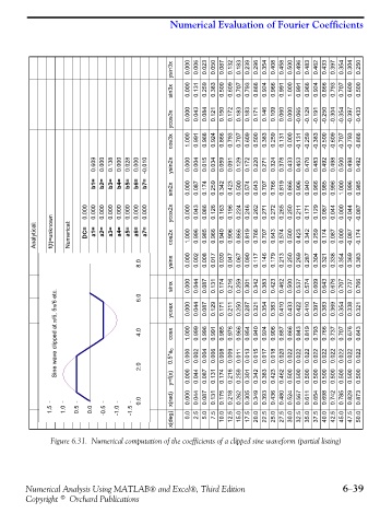
Figure 6.31. Numerical computation of the coefficients of a clipped sine waveform (partial listing)

Numerical Analysis Using MATLAB® and Excel®, Third Edition 6−39
Copyright © Orchard Publications