Page 261 - Numerical Analysis Using MATLAB and Excel

Chapter 6 Fourier, Taylor, and Maclaurin Series

(
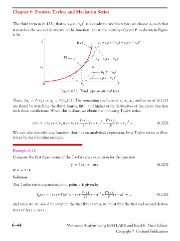
The third term in (6.122), that is, a v – v ) 0 2 is a quadratic and therefore, we choose a 2 such that
2
it matches the second derivative of the function iv() in the vicinity of point as shown in Figure
P
6.36.
i iv() a + a vv ) ( – 0 a v – v ) 0 2
( +
0
1
2
Pv i,( 0 0 ) a + a v – v ) 0
(
1
0
i 0 a 0
a vv ) ( – 0
1
a vv–( 2 0 ) 2

0 v 0 v

Figure 6.36. Third approximation of iv()

,
,
Then, 2a = i'' v ) ( 0 or a = i'' v ) ( 0 2 ⁄ . The remaining coefficients a a a 5 , and so on of (6.122)
4
3
2
2
are found by matching the third, fourth, fifth, and higher order derivatives of the given function
with these coefficients. When this is done, we obtain the following Taylor series.
i'' v ( ) i''' v ) (
0
0
iv() = iv ( 0 ) i' v ) ( + 0 ( v – v ) 0 -------------- vv ) ( + – 0 2 --------------- vv ) ( + – 0 3 + … (6.123)
2!
3!
We can also describe any function that has an analytical expression, by a Taylor series as illus-
trated by the following example.

Example 6.12
Compute the first three terms of the Taylor series expansion for the function

y = f x() = tan x (6.124)
at a = π . 4 ⁄

Solution:
The Taylor series expansion about point is given by
a
f'' a() 2 f''' a() 3
(
)
f x() = fa() + f' a() x – a + ------------ x –( 2! a ) + ------------- x –( 3! a ) + … (6.125)
n
and since we are asked to compute the first three terms, we must find the first and second deriva-
tives of fx() = tan . x

6−44 Numerical Analysis Using MATLAB® and Excel®, Third Edition
Copyright © Orchard Publications