Page 257 - Numerical Analysis Using MATLAB and Excel

Chapter 6 Fourier, Taylor, and Maclaurin Series

6.9 Power Series Expansion of Functions

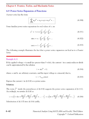
A power series has the form

∞
k
2
∑ a x = a + a x + a x + … (6.110)
k
0
2
1
k = 0
Some familiar power series expansions for real values of are
x
x
----- +
----- +
e = 1 + + x 2 x 3 x 4 … (6.111)
x
----- +
2! 3! 4!
x 3 x 5 x 7
sin x = x – ----- + ----- – ----- + … (6.112)
3! 5! 7!
x 2 x 4 x 6
cos x = 1 – ----- + ----- – ----- + … (6.113)
2! 4! 6!
The following example illustrates the fact that a power series expansion can lead us to a Fourier
Series.

Example 6.11

If the applied voltage is small (no greater than 5 volts), the current in a semiconductor diode
i
v
can be approximated by the relation
i = a e ( kv – 1 ) (6.114)

where and are arbitrary constants, and the input voltage is a sinusoid, that is,
a
k
v = V max cos ωt (6.115)

Express the current in (6.114) as a power series.
i
Solution:

The term e kv inside the parentheses of (6.114) suggests the power series expansion of (6.111).
Accordingly, we rewrite (6.114) as

3
2
4
2
3
4
)
)
)
)
)
)
kv
kv
kv
⎛
kv
⎛
kv
⎞
kv
i = a 1 + kv + ( ------------- + ( ------------- + ( ------------- + … 1 = akv + ( ------------- + ( ------------- + ( ------------- + … ⎞ (6.116)
–
⎝ 2! 3! 4! ⎠ ⎝ 2! 3! 4! ⎠
Substitution of (6.115) into (6.116) yields,
6−40 Numerical Analysis Using MATLAB® and Excel®, Third Edition
Copyright © Orchard Publications