Page 252 - Numerical Analysis Using MATLAB and Excel

Line Spectra

⁄
π k
A A π π ⎞ A
⎛
C = ------t = ------ --- + --- ⎠ = ---- (6.107)
⎝
2π
0
⁄
– π k 2π k k k
For the values for n ≠ 0 , integration of (6.106) yields
⁄
⁄
⁄
A – jnt π k A e jnπ k e – – jnπ k A ⎛ nπ ⎞
⋅
C = ---------------e – π k = ------ ------------------------------------- = ------ sin⋅ ⎝ ------
k ⎠
n
nπ
nπ
jn2π
⁄
j2
–
(6.108)
⁄
⁄
sin ( nπ k ) A sin ( nπ k )
⋅
= A-------------------------- = ---- --------------------------
⁄
nπ k nπ k
and thus,
∞ A sin ( nπ k )
⁄
⋅
ft() = ∑ ---- -------------------------- (6.109)
⁄
k
nπ k
n = – ∞
⁄
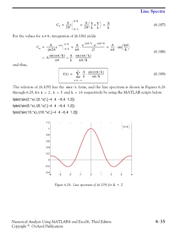
The relation of (6.109) has the sin x x form, and the line spectrum is shown in Figures 6.26
through 6.28, for k = 2 , k = 5 and k = 10 respectively by using the MATLAB scripts below.
fplot('sin(2.*x)./(2.*x)',[−4 4 −0.4 1.2])
fplot('sin(5.*x)./(5.*x)',[−4 4 −0.4 1.2])
fplot('sin(10.*x)./(10.*x)',[−4 4 −0.4 1.2])
1.2
K=2
1
0.8
0.6
0.4
0.2
0
-0.2
-0.4
-4 -3 -2 -1 0 1 2 3 4

Figure 6.26. Line spectrum of (6.109) for k = 2

Numerical Analysis Using MATLAB® and Excel®, Third Edition 6−35
Copyright © Orchard Publications