Page 251 - Numerical Analysis Using MATLAB and Excel

Chapter 6 Fourier, Taylor, and Maclaurin Series

Figure 6.24 shows the line spectrum for the half−wave rectification waveform of Example 6.6.

A/2
A/π DC
2 4 6 8

0 1 nωt

Figure 6.24. Line spectrum for half−wave rectifier of Example 6.6

The line spectra of other waveforms can be easily constructed from the Fourier series.

Example 6.10
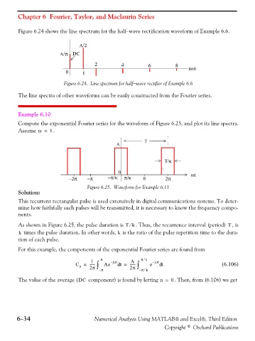
Compute the exponential Fourier series for the waveform of Figure 6.25, and plot its line spectra.
Assume ω = . 1

T
A

T/κ

0 ωt
−2π −π −π/κ π/κ π 2π
Figure 6.25. Waveform for Example 6.11
Solution:

This recurrent rectangular pulse is used extensively in digital communications systems. To deter-
mine how faithfully such pulses will be transmitted, it is necessary to know the frequency compo-
nents.

As shown in Figure 6.25, the pulse duration is Tk⁄ . Thus, the recurrence interval (period) , is
T
k
k times the pulse duration. In other words, is the ratio of the pulse repetition time to the dura-
tion of each pulse.
For this example, the components of the exponential Fourier series are found from

⁄
1 π – jnt A π k – jnt
C = ------ ∫ – π Ae t d = ------ ∫ – π k e t d (6.106)
2π
2π
n
⁄
The value of the average (DC component) is found by letting n = 0 . Then, from (6.106) we get

6−34 Numerical Analysis Using MATLAB® and Excel®, Third Edition
Copyright © Orchard Publications