Page 254 - Numerical Analysis Using MATLAB and Excel

Numerical Evaluation of Fourier Coefficients

whose period may be a day, a week, a month or even a year. In these situations, we need to eval-
uate the integral(s) using numerical integration.

The procedure presented here, will work for both the waveforms that have an analytical solution
and those that do not. Even though we may already know the Fourier series from analytical
methods, we can use this procedure to check our results.

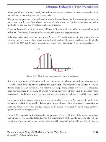
Consider the waveform of fx() shown in Figure 6.29, were we have divided it into small pulses of
width Δx . Obviously, the more pulses we use, the better the approximation.

If the time axis is in degrees, we can choose Δx to be 2.5° and it is convenient to start at the zero
point of the waveform. Then, using a spreadsheet, such as Microsoft Excel, we can divide the
period 0° to 360° in 2.5° intervals, and enter these values in Column of the spreadsheet.
A
fx()

x

Figure 6.29. Waveform whose analytical expression is unknown

Since the arguments of the sine and the cosine are in radians, we multiply degrees by π
(3.1459...) and divide by 180 to perform the conversion. We enter these in Column and we
B
x
C
denote them as . In Column we enter the corresponding values of y = f x() as measured
from the waveform. In Columns and we enter the values of cos x and the product ycos x
E
D
respectively. Similarly, we enter the values of sin x and ysin x in Columns and respectively.
F
G
π
Next, we form the sums of ycos x and ysin x , we multiply these by Δx , and we divide by to
obtain the coefficients a 1 and b 1 . To compute the coefficients of the higher order harmonics, we
form the products ycos 2x , ysin 2x , ycos 3x , ysin 3x , and so on, and we enter these in subse-
quent columns of the spreadsheet.

Figure 6.30 is a partial table showing the computation of the coefficients of the square waveform,
and Figure 6.31 is a partial table showing the computation of the coefficients of a clipped sine
waveform. The complete tables extend to the seventh harmonic to the right and to 360° down.

Numerical Analysis Using MATLAB® and Excel®, Third Edition 6−37
Copyright © Orchard Publications