Page 260 - Numerical Analysis Using MATLAB and Excel

Taylor and Maclaurin Series

i
iv()

Pv i,( 0 0 )

i 0 a 0

0 v v
0
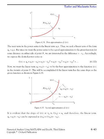
Figure 6.34. First approximation of iv()

The next term in the power series is the linear term a x . Thus, we seek a linear term of the form
1
a + a x . But since we want the power series to be a good approximation to the given function for
1
0
P
some distance on either side of point , we are interested in the difference v – v 0 . Accordingly,
we express the desired power series as

(
fv() = a + a v – v ) 0 a vv ) ( + – 0 2 a vv ) ( + – 0 3 a v – v ) 0 4 + … (6.122)
( +
1
2
3
4
0
Now, we want the linear term a + a vv ) ( – 0 to be the best approximation to the function iv()
0
1
in the vicinity of point . This will be accomplished if the linear term has the same slope as the
P
given function as shown in Figure 6.35.
i
iv()
Pv i,( 0 0 ) a + a v – v ) 0
(
0
0
i 0 a 0
a vv–( 0 0 )

0 v 0 v
Figure 6.35. Second approximation of iv()

It is evident that the slope of iv() at v 0 is i' v ) ( 0 = a 1 and therefore, the linear term
a + a vv ) ( – 0 can be expressed as iv( 0 ) i' v ) ( + 0 ( vv 0 . )
–
1
0

Numerical Analysis Using MATLAB® and Excel®, Third Edition 6−43
Copyright © Orchard Publications