Page 314 - Numerical Analysis and Modelling in Geomechanics

F.BASILE 295

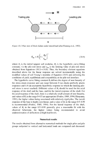
Figure 10.1 Plan view of block failure under lateral load (after Fleming et al., 1992).

(10.9)

where E i is the initial tangent soil modulus, R f is the hyperbolic curve-fitting
constant, t is the pile-soil stress and t lim is the limiting value of pile-soil stress
obtained from Equations (10.3)−(10.8). Thus, the boundary element equations
described above for the linear response are solved incrementally using the
modified values of soil Young’s modulus of Equation (10.9) and enforcing the
conditions of yield, equilibrium and compatibility at the pile-soil interface.
The hyperbolic curve fitting constant R defines the degree of non-linearity of
f
the stress-strain response and can range between 0 (an elastic-perfectly plastic
response) and 1.0 (an asymptotic hyperbolic response in which the limiting pile-
soil stress is never reached). Different values of R should be used for the axial
f
response of the shaft and the base, and for the lateral response of the shaft. For
the axial response of the shaft, there is a relatively small amount of non-linearity,
and values of R in the range 0–0.5 are appropriate (Poulos, 1989, 1994; Hirayama,
f
1991), the higher values being associated with relatively rigid piles. The (axial)
response of the base is highly non-linear, and a value of R in the range 0.9–0.99
f
is recommended (Poulos, 1989, 1994). For the lateral response of the shaft,
values of R f in the range 0.5–0.99 generally give a reasonable fit with the
observed behaviour, the higher values being recommended to avoid
underestimation of deflections at high load levels.

Numerical results
The results obtained from alternative numerical methods for single piles and pile
groups subjected to vertical and horizontal loads are compared and discussed.