Page 62 - Numerical Analysis and Modelling in Geomechanics

COMPRESSED AIR TUNNELLING 43

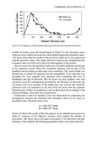
Figure 2.8 Comparison of the predicted and measured air losses from the tunnel face.

number of sections along the tunnel length. In Figure 2.8, the calculated values
of the air losses at these locations have been plotted against the measured values.
The figure shows that the results of the numerical model are in close agreement
with the measured values. The slight differences between the calculated and the
measured values are likely to be due to the heterogeneity of the ground.
The air losses from the perimeter walls were calculated using the second part
of the numerical model where the excavation sequence and the age of the
installed shotcrete lining at each stage were considered. The tunnel length was
divided into a number of segments and the permeability of the shotcrete was
calculated for each segment from equation (2.8) considering the time of
installation and age of shotcrete. The air losses for each segment were then
calculated using the corresponding permeability and thickness of shotcrete and
soil layers. For every location of the tunnel face, the total air loss from the
perimeter walls was considered as the sum of the air losses from the segments
behind the face. Delays in construction, such as those due to local collapse of the
tunnel or holidays, were taken into consideration.
Coefficients A and B in equation (2.8) were determined by minimising the
discrepancies between the measured and calculated values of air losses as
described earlier. The final values were:

Figure 2.9 shows the results of the GA analysis in the identification process in
terms of variation of the objective function value against the number of
generations. The figure shows the rapid convergence of the algorithm and high
efficiency of the method. The following parameter values were used in the GA: