Page 332 - Numerical Methods for Chemical Engineering

The theory of probability 321

where P(E 2 |E 1 )isthe conditional probability that if E 1 occurs, so does E 2 . If the probability
of observing event E 2 does not depend upon whether E 1 occurs or not, the two events are
said to be independent, and

P(E 2 |E 1 ) = P(E 2 ) P(E 1 ∩ E 2 ) = P(E 1 )P(E 2 ) (7.9)

The conditional and joint probabilities are related by Bayes’ theorem, whose application to
statistics forms the basis of the next chapter,

P(E 1 ∩ E 2 ) = P(E 1 )P(E 2 |E 1 ) = P(E 2 )P(E 1 |E 2 ) (7.10)
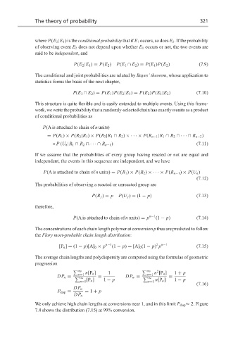
This structure is quite flexible and is easily extended to multiple events. Using this frame-
work, we write the probability that a randomly-selected chain has exactly n units as a product
of conditional probabilities as
P(A is attached to chain of n units)
= P(R 1 ) × P(R 2 |R 1 ) × P(R 3 |R 1 ∩ R 2 ) ×···× P(R n−1 |R 1 ∩ R 2 ∩···∩ R n−2 )

×P (U n |R 1 ∩ R 2 ∩···∩ R n−1 ) (7.11)

If we assume that the probabilities of every group having reacted or not are equal and
independent, the events in this sequence are independent, and we have

P(A is attached to chain of n units) = P(R 1 ) × P(R 2 ) ×···× P(R n−1 ) × P(U n )
(7.12)
The probabilities of observing a reacted or unreacted group are

P(R j ) = p P(U j ) = (1 − p) (7.13)

therefore,

P(A is attached to chain of n units) = p n−1 (1 − p) (7.14)

The concentrations of each chain length polymer at conversion p thus are predicted to follow
the Flory most-probable chain length distribution:

2 n−1
[P n ] = (1 − p)[A] 0 × p n−1 (1 − p) = [A] 0 (1 − p) p (7.15)
The average chain lengths and polydispersity are computed using the formulas of geometric
progression
∞ n[P n ] 1 ∞ n [P n ] 1 + p
2
n=1 n=1
∞ [P n ] 1 − p ∞ n[P n ] 1 − p
DP n ≡ = DP w ≡ =
n=1 n=1
(7.16)
DP w
P disp ≡ = 1 + p
DP n
We only achieve high chain lengths at conversions near 1, and in this limit P disp ≈ 2. Figure
7.4 shows the distribution (7.15) at 99% conversion.