Page 337 - Numerical Methods for Chemical Engineering

326 7 Probability theory and stochastic simulation

2

1
1
1

12
w
1

2

2 1
cnversin
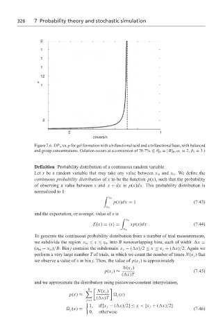
Figure 7.6 DP w vs. p for gel formation with a bifunctional acid and a trifunctional base, with balanced
end group concentrations. Gelation occurs at a conversion of 70.7%. ([A] 0 = [B] 0 ,α 1 = 2,β 2 = 3.)

Definition Probability distribution of a continuous random variable
Let x be a random variable that may take any value between x lo and x hi . We define the
continuous probability distribution of x to be the function p(x), such that the probability
of observing a value between x and x + dx is p(x)dx. This probability distribution is
normalized to 1:
'
x hi
p(x)dx = 1 (7.43)
x lo
and the expectation, or average, value of x is
'
x hi
E(x) = x = xp(x)dx (7.44)
x lo
To generate the continuous probability distribution from a number of trial measurements,
we subdivide the region x lo ≤ x ≤ x hi into B nonoverlapping bins, each of width x =
(x hi − x lo )/B. Bin j contains the subdomain x j − ( x)/2 ≤ x ≤ x j + ( x)/2. Again we
perform a very large number T of trials, in which we count the number of times N(x j ) that
we observe a value of x in bin j. Then, the value of p(x j ) is approximately
N(x j )
p(x j ) ≈ (7.45)
( x)T
and we approximate the distribution using piecewise-constant interpolation,
B
N(x j )
p(x) ≈ j (x)
( x)T
j=1
1, if [x j − ( x)/2] ≤ x < [x j + ( x)/2]

j (x) = (7.46)
0, otherwise