Page 341 - Numerical Methods for Chemical Engineering

330 7 Probability theory and stochastic simulation

n
n n 1 n 2 n n

1 1
1 2
11
1 1
2 1
1
11

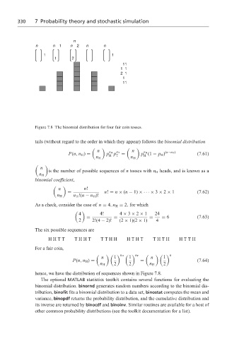
Figure 7.8 The binomial distribution for four fair coin tosses.

tails (without regard to the order in which they appear) follows the binomial distribution

n n (n−n H )
n H
n H
P(n, n H ) = p p T n T = p (1 − p H ) (7.61)
H
H
n H n H

n
is the number of possible sequences of n tosses with n H heads, and is known as a
n H
binomial coefficient,

n n!
= n! = n × (n − 1) × ··· × 3 × 2 × 1 (7.62)
n H !(n − n H )!
n H
As a check, consider the case of n = 4, n H = 2, for which

4 4! 4 × 3 × 2 × 1 24
= = = = 6 (7.63)
2 2!(4 − 2)! (2 × 1)(2 × 1) 4
The six possible sequences are
HHTT THHT TTHH HTHT THTH HTTH
For a fair coin,
n 1 1 n 1
n H n T n
P(n, n H ) = = (7.64)
n H 2 2 n H 2
hence, we have the distribution of sequences shown in Figure 7.8.
The optional MATLAB statistics toolkit contains several functions for evaluating the
binomial distribution. binornd generates random numbers according to the binomial dis-
tribution, binofit fits a binomial distribution to a data set, binostat computes the mean and
variance, binopdf returns the probability distribution, and the cumulative distribution and
its inverse are returned by binocdf and binoinv. Similar routines are available for a host of
other common probability distributions (see the toolkit documentation for a list).