Page 345 - Numerical Methods for Chemical Engineering

334 7 Probability theory and stochastic simulation

In MATLAB, we generate a random number distributed according to N(0, 1) using randn.

From such a random number r, we obtain a random number r distributed according to
2
N(µ, σ ) from the rule

r = µ + σr (7.87)
or we can use the statistics toolkit function normrnd to directly generate random numbers
2
from N(µ, σ ). Both randn and normrnd can also generate matrices of independent random
numbers.

The Poisson distribution
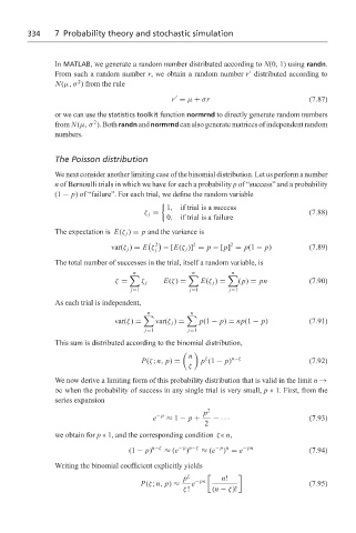
We next consider another limiting case of the binomial distribution. Let us perform a number
n of Bernoulli trials in which we have for each a probability p of “success” and a probability
(1 − p) of “failure”. For each trial, we define the random variable

1, if trial is a success
ζ j = (7.88)
0, if trial is a failure
The expectation is E(ζ j ) = p and the variance is
2
2 2
var(ζ j ) = E ζ − [E(ζ j )] = p − [p] = p(1 − p) (7.89)
j
The total number of successes in the trial, itself a random variable, is
n n n

ζ = ζ j E(ζ) = E(ζ j ) = (p) = pn (7.90)
j=1 j=1 j=1
As each trial is independent,
n n

var(ζ) = var(ζ j ) = p(1 − p) = np(1 − p) (7.91)
j=1 j=1
This sum is distributed according to the binomial distribution,

n ζ n−ζ
P(ζ; n, p) = p (1 − p) (7.92)
ζ
We now derive a limiting form of this probability distribution that is valid in the limit n →
∞ when the probability of success in any single trial is very small, p 1. First, from the
series expansion
p 2
−p
e ≈ 1 − p + − ··· (7.93)
2
we obtain for p 1, and the corresponding condition ζ n,
(1 − p) n−ζ ≈ (e −p n−ζ ≈ (e −p n −pn (7.94)
) = e
)
Writing the binomial coefficient explicitly yields
p ζ −pn n!
P(ζ; n, p) ≈ e (7.95)
ζ! (n − ζ)!