Page 344 - Numerical Methods for Chemical Engineering

Important probability distributions 333

1
σ = 2
σ =
1 σ = 1

12

1

assian raiit distritin

2

− −2 −1 1 2

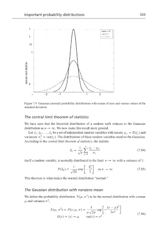
Figure 7.9 Gaussian (normal) probability distributions with means of zero and various values of the
standard deviation.

The central limit theorem of statistics
We have seen that the binomial distribution of a random walk reduces to the Gaussian
distribution as n →∞. We now make this result more general.
Let ζ 1 ,ζ 2 ,...,ζ n be a set of independent random variables with means µ j = E(ζ j ) and
2
variances σ = var(ζ j ). The distributions of these random variables need not be Gaussian.
j
According to the central limit theorem of statistics, the statistic
n
1 ζ j − µ j
S n = √ (7.84)
n σ j
j=1
itself a random variable, is normally distributed in the limit n →∞ with a variance of 1:
1 S n 2
P(S n ) = √ exp − as n →∞ (7.85)
2π 2

This theorem is what makes the normal distribution “normal.”

The Gaussian distribution with nonzero mean
2
We define the probability distribution N(µ, σ ) to be the normal distribution with a mean
2
µ and variance σ ,
1 (x − µ) 2
2
N(µ, σ ) = P(x; µ, σ) = √ exp − 2
σ 2π 2σ (7.86)
E(x) = x = µ var(x) = σ 2