Page 457 - Numerical Methods for Chemical Engineering

446 9 Fourier analysis

a
2
t
2

1 2
t

w 2 w a 12
2
w w 1
w 2 w a 2
1
w 2 w a 1
1 1 2 2
w

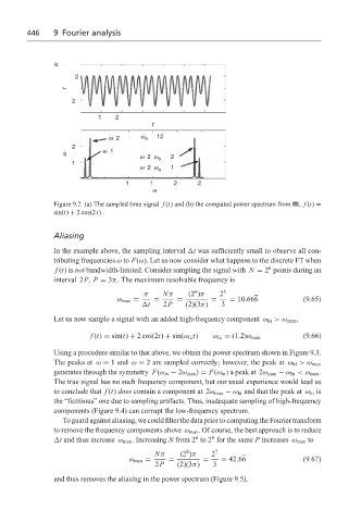
Figure 9.2 (a) The sampled time signal f (t) and (b) the computed power spectrum from fft, f (t) =
sin(t) + 2 cos(2t).

Aliasing

In the example above, the sampling interval t was sufficiently small to observe all con-
tributing frequencies ω to F(ω). Let us now consider what happens to the discrete FT when
6
f (t)is not bandwidth-limited. Consider sampling the signal with N = 2 points during an
interval 2P, P = 3π. The maximum resolvable frequency is
6
π Nπ (2 )π 2 5
ω max = = = = = 10.666 (9.65)
t 2P (2)(3π) 3
Let us now sample a signal with an added high-frequency component ω hi >ω max ,

f (t) = sin(t) + 2 cos(2t) + sin(ω hi t) ω hi = (1.2)ω max (9.66)
Using a procedure similar to that above, we obtain the power spectrum shown in Figure 9.3.

The peaks at ω = 1 and ω = 2 are sampled correctly; however, the peak at ω hi >ω max
generates through the symmetry F(ω m − 2ω max ) = F(ω m ) a peak at 2ω max − ω hi <ω max .
The true signal has no such frequency component, but our usual experience would lead us
to conclude that f (t) does contain a component at 2ω max − ω hi and that the peak at ω hi is
the “fictitious” one due to sampling artifacts. Thus, inadequate sampling of high-frequency
components (Figure 9.4) can corrupt the low-frequency spectrum.
To guard against aliasing, we could filter the data prior to computing the Fourier transform
to remove the frequency components above ω max . Of course, the best approach is to reduce
8
6
t and thus increase ω max . Increasing N from 2 to 2 for the same P increases ω max to
8
Nπ (2 )π 2 7
ω max = = = = 42.66 (9.67)
2P (2)(3π) 3
and thus removes the aliasing in the power spectrum (Figure 9.5).