Page 459 - Numerical Methods for Chemical Engineering

448 9 Fourier analysis

2
t
2

1 1 2
t

w 2 w a 2
w 1
w
w i
2
2 1
w
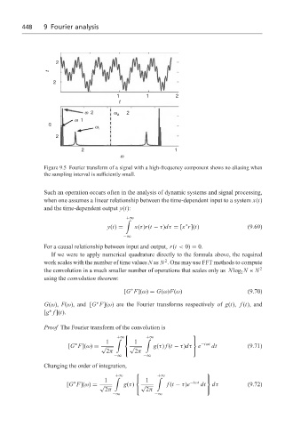
Figure 9.5 Fourier transform of a signal with a high-frequency component shows no aliasing when
the sampling interval is sufficiently small.

Such an operation occurs often in the analysis of dynamic systems and signal processing,
when one assumes a linear relationship between the time-dependent input to a system x(t)
and the time-dependent output y(t):
+∞
'
∗
y(t) = x(τ)r(t − τ)dτ = [x r](t) (9.69)
−∞
For a causal relationship between input and output, r(t < 0) = 0.
If we were to apply numerical quadrature directly to the formula above, the required
2
work scales with the number of time values N as N . One may use FFT methods to compute
the convolution in a much smaller number of operations that scales only as Nlog N « N 2
2
using the convolution theorem:
[G F](ω) = G(ω)F(ω) (9.70)
∗
G(ω), F(ω), and [G F](ω) are the Fourier transforms respectively of g(t), f (t), and
∗
[g f ](t).
∗
Proof The Fourier transform of the convolution is

 
+∞ +∞
1 '  1 ' 
∗ −iωt
[G F](ω) = √ √ g(τ) f (t − τ)dτ e dt (9.71)
2π  2π 
−∞ −∞
Changing the order of integration,
 
+∞ +∞
'
'
1  1 
∗ −iωt
[G F](ω) = √ g(τ) √ f (t − τ)e dt dτ (9.72)
2π  2π 
−∞ −∞