Page 463 - Numerical Methods for Chemical Engineering

452 9 Fourier analysis

−
1
1 1
1

1 2
1

−1
−2
−
2 1 12

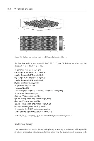
Figure 9.6 Surface and contour plots of a 2-D periodic function f (x, y).

that has four peaks at (q x , q y ) = (1, 0), (3, 0), (1, 2), and (0, 4) from sampling over the
domain 0 ≤ x < 4π, 0 ≤ y < 4π,

% generate real-space (x,y) grid
P x = 2*pi; N x = 2ˆ6; dx = 2*P x/N x;
x val = linspace(0, 2*P x - dx, N x);
P y = 2*pi; N y = 2ˆ6; dy = 2*P y/N y;
y val = linspace(0, 2*P y-dy,N y);
[X,Y] = meshgrid(x val,y val);
% generate f(x,y) values
F = zeros(size(X));
F=F+ cos(X) + cos(3.*X) + 2*sin(X).*cos(2.*Y) + cos(4.*Y);
% generate the q-space grid
dq x = pi/P x; q x max = pi/dx;
q x val = linspace(0, 2*q x max-dq x, N x);
dq y = pi/P y; q y max = pi/dy;
q y val = linspace(0, 2*q y max-dq y, N y);
[QX,QY] = meshgrid(q x val, q y val);
% compute the 2-D FT and power spectrum
F FT = (dx*dy/2/pi).*fft2(F); F PS = abs(F FT);
Plots of f (x, y) and |F(q x , q y )| are shown in Figure 9.6 and Figure 9.7.

Scattering theory

This section introduces the theory underpinning scattering experiments, which provide
structural information about materials from observing the interaction of a sample with