Page 470 - Numerical Methods for Chemical Engineering

Problems 459

1

1
n
2
1 1
q derees
1 2
A A
1 1
s en n 1

1 1
2
q derees
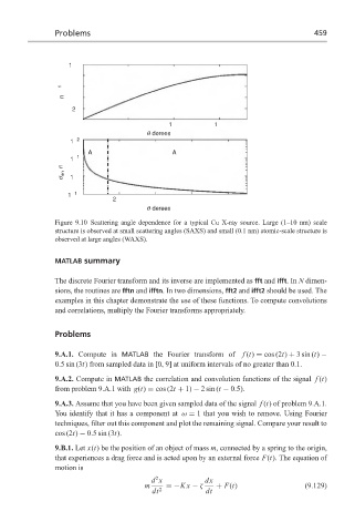
Figure 9.10 Scattering angle dependence for a typical Cu X-ray source. Large (1–10 nm) scale
structure is observed at small scattering angles (SAXS) and small (0.1 nm) atomic-scale structure is
observed at large angles (WAXS).

MATLAB summary

The discrete Fourier transform and its inverse are implemented as fft and ifft.In N dimen-
sions, the routines are fftn and ifftn. In two dimensions, fft2 and ifft2 should be used. The
examples in this chapter demonstrate the use of these functions. To compute convolutions
and correlations, multiply the Fourier transforms appropriately.

Problems

9.A.1. Compute in MATLAB the Fourier transform of f (t) = cos (2t) + 3 sin (t) −
0.5 sin (3t) from sampled data in [0, 9] at uniform intervals of no greater than 0.1.

9.A.2. Compute in MATLAB the correlation and convolution functions of the signal f (t)
from problem 9.A.1 with g(t) = cos (2t + 1) − 2 sin (t − 0.5).

9.A.3. Assume that you have been given sampled data of the signal f (t) of problem 9.A.1.
You identify that it has a component at ω = 1 that you wish to remove. Using Fourier
techniques, filter out this component and plot the remaining signal. Compare your result to
cos (2t) − 0.5 sin (3t).
9.B.1. Let x(t) be the position of an object of mass m, connected by a spring to the origin,
that experiences a drag force and is acted upon by an external force F(t). The equation of
motion is
2
d x dx
m =−Kx − ζ + F(t) (9.129)
dt 2 dt