Page 176 - Numerical methods for chemical engineering

162 4 Initial value problems

Newton–Cotes integration

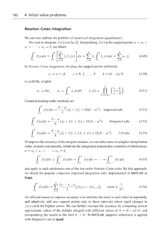
We can now address the problem of numerical integration (quadrature).
We want to integrate f (x)over[a, b]. Interpolating f (x) at the support points a = x 0 <
x 1 < ··· < x N = b, we obtain

b N N b N
' ' '
b

f (x)dx ≈ f j L j (x) dx = f j L j (x)dx = w j f j (4.49)
a a j=0 j=0 a j=0
In Newton–Cotes integration, we place the support points uniformly,
x j = a + jh j = 0, 1,..., N h = (b − a)/N (4.50)
to yield the weights

N N
'
0 t − k
w j = hα j α j = L j (t)dt L j (t) = (4.51)
0 k=0,k = j j − k
Common leading-order methods are
' b
b − a 3
f (x)dx = { f 0 + f 1 }+ O(|b − a| ) trapezoid rule (4.52)
a 2
b − a 4
' b
f (x)dx = { f 0 + 4 f 1 + f 2 }+ O(|b − a| ) Simpson’s rule (4.53)
a 6
b − a 5
' b
f (x)dx = { f 0 + 3 f 1 + 3 f 2 + f 3 }+ O(|b − a| ) 3/8 rule (4.54)
a 8
To improve the accuracy of the integral estimate, we can either move to a higher interpolation
order, or more conveniently, subdivide the integration domain into a number of subdomains,
a = x 0 < x 1 < ··· < x N = b,
' b ' x 1 ' x 2 ' x N
f (x)dx = f (x)dx + f (x)dx +· · · + f (x)dx (4.55)
a x 0 x 1 x N−1
and apply to each subdomain one of the low-order Newton–Cotes rules. By this approach,
we obtain the popular composite trapezoid integration rule, implemented in MATLAB as
trapz,

b N
'
(x j − x j−1 ) 1
f (x)dx ≈ [ f (x j ) + f (x j−1 )] error ∝ (4.56)
a j=1 2 N 2
An efficient means to improve accuracy is to estimate the error in each interval separately,
and adaptively add new support points only to those intervals where rapid changes in
f (x) yield the highest errors. We can further increase the accuracy by computing several
approximate values of the definite integral with different values of h = (b − a)/N, and
extrapolating the results to the limit h → 0.In MATLAB, adaptive refinement is applied
with Simpson’s rule in quad.