Page 175 - Numerical methods for chemical engineering

Polynomial interpolation 161

1

2
1

1 1 2 2

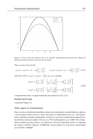
Figure 4.2 Plot of the sine function f(x) at its Hermite interpolating polynomial p(x), fitting the
function and first derivative values at each end point.

Thus, we have from (4.44)
2 2

x − b x − a
L 01 (x) = l 01 (x) = (x − a) L 11 (x) = l 01 (x) = (x − b) (4.47)
a − b b − a
(1)
and from (4.45), L j0 (x) = l j0 (x) − l (x j )L j0 (x), yielding
j0
2
2
x − b 2 x − b

L 00 (x) = − (x − a)
a − b (a − b) a − b
(4.48)
2
2

x − a 2 x − a
L 01 (x) = − (x − b)
b − a (b − a) b − a
Using hermite ex.m, we approximate the sine function on [0, π]by
hermite ex(‘sin’,0,pi);
to generate Figure 4.2.

Other types of interpolation

Here, we have considered interpolation using only polynomials to match function values at
a set of support points; however, many other types of interpolation exist, e.g. with trigono-
metric functions instead of polynomials. For brevity, we do not consider these methods here,
but refer the interested reader to Press et al. (1992) and Quateroni et al. (2000). The interpo-
lation methods introduced above are sufficient to meet our immediate needs of computing
the values of definite integrals. In MATLAB, various options for polynomial interpolation
are available in interp1.