Page 170 - Numerical methods for chemical engineering

156 4 Initial value problems

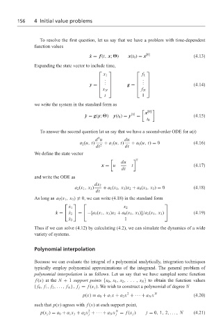
To resolve the first question, let us say that we have a problem with time-dependent
function values
˙ x = f (t, x; Θ) x(t 0 ) = x [0] (4.13)

Expanding the state vector to include time,
   
x 1 f 1
 .   . 
. .
 .   .  (4.14)
 g =  
y = 
x N f N
   
t 1
we write the system in the standard form as
[0]
x
[0]
˙ y = g(y; Θ) y(t 0 ) = y = (4.15)
t 0
To answer the second question let us say that we have a second-order ODE for u(t)
2
d u du
a 2 (u, t) + a 1 (u, t) + a 0 (u, t) = 0 (4.16)
dt 2 dt
We define the state vector
T

du
x = u t (4.17)
dt
and write the ODE as
dx 2
a 2 (x 1 , x 3 ) + a 1 (x 1 , x 3 )x 2 + a 0 (x 1 , x 3 ) = 0 (4.18)
dt
As long as a 2 (x 1 , x 3 ) = 0, we can write (4.18) in the standard form

   
˙ x 1 x 2
˙ x =  ˙ x 2  =  −[a 1 (x 1 , x 3 )x 2 + a 0 (x 1 , x 3 )]/a 2 (x 1 , x 3 )  (4.19)
1
˙ x 3
Thus if we can solve (4.12) by calculating (4.2), we can simulate the dynamics of a wide
variety of systems.

Polynomial interpolation

Because we can evaluate the integral of a polynomial analytically, integration techniques
typically employ polynomial approximations of the integrand. The general problem of
polynomial interpolation is as follows. Let us say that we have sampled some function
f (x)atthe N + 1 support points {x 0 , x 1 , x 2 ,..., x N } to obtain the function values
{ f 0 , f 1 , f 2 ,..., f N } , f j = f (x j ). We wish to construct a polynomial of degree N
2
p(x) = a 0 + a 1 x + a 2 x + ··· + a N x N (4.20)
such that p(x) agrees with f (x) at each support point,
2
p(x j ) = a 0 + a 1 x j + a 2 x +· · · + a N x N = f (x j ) j = 0, 1, 2,..., N (4.21)
j j