Page 173 - Numerical methods for chemical engineering

Polynomial interpolation 159

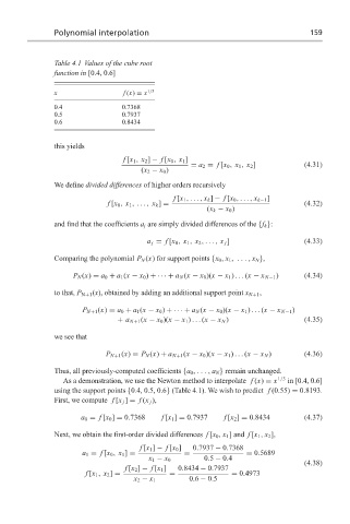
Table 4.1 Values of the cube root
function in [0.4, 0.6]

x f (x) = x 1/3
0.4 0.7368
0.5 0.7937
0.6 0.8434

this yields
f [x 1 , x 2 ] − f [x 0 , x 1 ]
= a 2 ≡ f [x 0 , x 1 , x 2 ] (4.31)
(x 2 − x 0 )
We define divided differences of higher orders recursively
f [x 1 ,..., x k ] − f [x 0 ,..., x k−1 ]
f [x 0 , x 1 , . .., x k ] = (4.32)
(x k − x 0 )
and find that the coefficients a j are simply divided differences of the {f k }:

a j = f [x 0 , x 1 , x 2 ,..., x j ] (4.33)

Comparing the polynomial P N (x) for support points {x 0 , x 1 , ..., x N },

P N (x) = a 0 + a 1 (x − x 0 ) +· · · + a N (x − x 0 )(x − x 1 ) ... (x − x N−1 ) (4.34)
to that, P N+1 (x), obtained by adding an additional support point x N+1 ,

P N+1 (x) = a 0 + a 1 (x − x 0 ) + ··· + a N (x − x 0 )(x − x 1 ) ... (x − x N−1 )
+ a N+1 (x − x 0 )(x − x 1 ) ... (x − x N ) (4.35)

we see that
P N+1 (x) = P N (x) + a N+1 (x − x 0 )(x − x 1 ) ... (x − x N ) (4.36)

Thus, all previously-computed coefficients {a 0 ,..., a N } remain unchanged.
As a demonstration, we use the Newton method to interpolate f (x) = x 1/3 in [0.4, 0.6]
using the support points {0.4, 0.5, 0.6} (Table 4.1). We wish to predict f (0.55) = 0.8193.
First, we compute f [x j ] = f (x j ),

a 0 = f [x 0 ] = 0.7368 f [x 1 ] = 0.7937 f [x 2 ] = 0.8434 (4.37)

Next, we obtain the first-order divided differences f [x 0 , x 1 ] and f [x 1 , x 2 ],
f [x 1 ] − f [x 0 ] 0.7937 − 0.7368
a 1 = f [x 0 , x 1 ] = = = 0.5689
x 1 − x 0 0.5 − 0.4
(4.38)
f [x 2 ] − f [x 1 ] 0.8434 − 0.7937
f [x 1 , x 2 ] = = = 0.4973
x 2 − x 1 0.6 − 0.5