Page 172 - Numerical methods for chemical engineering

158 4 Initial value problems

a
2
1

−2
−
− 1 1

2
12
1 a rane inter atin

1

a reeent at sr t ints

1 1

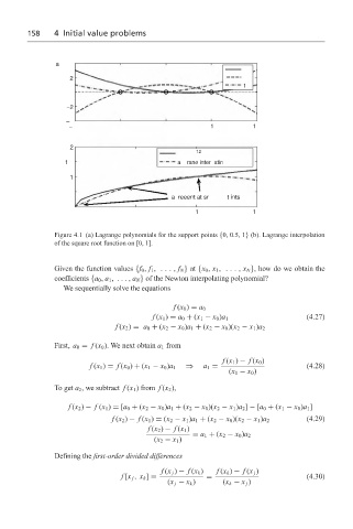
Figure 4.1 (a) Lagrange polynomials for the support points {0, 0.5, 1} (b). Lagrange interpolation
of the square root function on [0, 1].

Given the function values {f 0 , f 1 , ..., f N } at {x 0 , x 1 , ..., x N }, how do we obtain the
coefficients {a 0 , a 1 , ..., a N } of the Newton interpolating polynomial?
We sequentially solve the equations

f (x 0 ) = a 0
f (x 1 ) = a 0 + (x 1 − x 0 )a 1 (4.27)
f (x 2 ) = a 0 + (x 2 − x 0 )a 1 + (x 2 − x 0 )(x 2 − x 1 )a 2
First, a 0 = f (x 0 ). We next obtain a 1 from

f (x 1 ) − f (x 0 )
f (x 1 ) = f (x 0 ) + (x 1 − x 0 )a 1 ⇒ a 1 = (4.28)
(x 1 − x 0 )

To get a 2 , we subtract f (x 1 ) from f (x 2 ),

f (x 2 ) − f (x 1 ) = [a 0 + (x 2 − x 0 )a 1 + (x 2 − x 0 )(x 2 − x 1 )a 2 ] − [a 0 + (x 1 − x 0 )a 1 ]
(4.29)
f (x 2 ) − f (x 1 ) = (x 2 − x 1 )a 1 + (x 2 − x 0 )(x 2 − x 1 )a 2
f (x 2 ) − f (x 1 )
= a 1 + (x 2 − x 0 )a 2
(x 2 − x 1 )
Defining the first-order divided differences
f (x j ) − f (x k ) f (x k ) − f (x j )
f [x j , x k ] = = (4.30)
(x j − x k ) (x k − x j )