Page 174 - Numerical methods for chemical engineering

160 4 Initial value problems

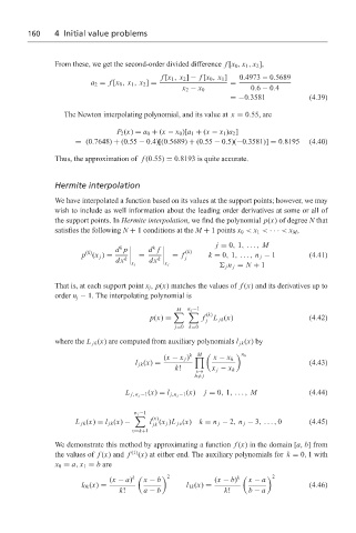
From these, we get the second-order divided difference f [x 0 , x 1 , x 2 ],
f [x 1 , x 2 ] − f [x 0 , x 1 ] 0.4973 − 0.5689
a 2 = f [x 0 , x 1 , x 2 ] = =
x 2 − x 0 0.6 − 0.4
=−0.3581 (4.39)
The Newton interpolating polynomial, and its value at x = 0.55, are

P 2 (x) = a 0 + (x − x 0 )[a 1 + (x − x 1 )a 2 ]
= (0.7648) + (0.55 − 0.4)[(0.5689) + (0.55 − 0.5)(−0.3581)] = 0.8195 (4.40)

Thus, the approximation of f (0.55) = 0.8193 is quite accurate.

Hermite interpolation
We have interpolated a function based on its values at the support points; however, we may
wish to include as well information about the leading order derivatives at some or all of
the support points. In Hermite interpolation, we find the polynomial p(x) of degree N that
satisfies the following N + 1 conditions at the M + 1 points x 0 < x 1 < ··· < x M ,

j = 0, 1, ..., M
k k
(k) d p d f (k)
p (x j ) = = = f j k = 0, 1,. . . , n j − 1 (4.41)
dx k dx k
x j x j j n j = N + 1
That is, at each support point x j , p(x) matches the values of f (x) and its derivatives up to
order n j − 1. The interpolating polynomial is
M n j −1
(k)
p(x) = f j L jk (x) (4.42)
j=0 k=0

where the L jk (x) are computed from auxiliary polynomials l jk (x)by
M
(x − x j ) k 0 x − x h n h
l jk (x) = (4.43)
k! x j − x h
h=0
h = j
L j, n j −1 (x) = l j,n j −1 (x) j = 0, 1, ..., M (4.44)

n j −1
(v)
L jk (x) = l jk (x) − l (x j )L jv (x) k = n j − 2, n j − 3,. . . , 0 (4.45)
jk
v=k+1
We demonstrate this method by approximating a function f (x) in the domain [a, b] from
the values of f (x) and f (1) (x) at either end. The auxiliary polynomials for k = 0, 1 with
x 0 = a, x 1 = b are
(x − a) k x − b 2 (x − b) k x − a 2
l 0k (x) = l 1k (x) = (4.46)
k! a − b k! b − a