Page 142 - Organic Electronics in Sensors and Biotechnology

Integrated Pyr oelectric Sensors 119

to 1/e. The distribution of the local resistivity of the capacitive layer
is described by
ρ() = ρ( )e x / δ (4.2)
0
x
where ρ(0) = resistivity at interface (depth x = 0).
The phase of the Young element is frequency-dependent. How-
ever, for small values of p it can be approximated by the following
expressions, of which the second is a frequency-independent value.
⎛ 1 ⎞
°
° − )p
φ ≈−90 1 − ln( ωτ + p −1 ⎟ ⎠ ≈−90 1 ( (4.3)
⎜
⎝
)
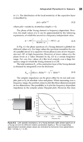
In Fig. 4.1 the phase spectrum of a Young element is plotted for
different values of p. For large values the spectrum resembles the one
of a parallel circuit of a capacitor whose phase is zero at low frequen-
cies and −90° at high frequencies. However, at lower values of p, the
phase levels at a value obtained by Eq. 4.3 in a certain frequency
range. For very low values of p this level extends over a large fre-
quency range in which the Young element is a CPE.
The total resistance R of the conduction layer of the Young element
tot
is obtained by integration over the thickness:
d p<<1
=
R tot ∫ dR x = R()( e 1 / p − ) ≈ R() e 1 /p (4.4)
1
)
(
0
0
0
The complex impedance can be given either by its real and com-
plex part or by its absolute value and phase. When measuring over a
frequency range, the problem arises to plot this three-dimensional plot
in two dimensions. One possibility is to plot the frequency-dependent
impedance in the complex plane (Nyquist plot). However, this does
0
–10
Conductivity
–20
δ = p d
–30 p = 50%
Phase (deg) –50
d –40 –45°
–60 p = 15%
–70
Resistivity –77.5°
–80 p = 5% –85°
–90
1.E+01 1.E+02 1.E+03 1.E+04 1.E+05 1.E+06
Frequency (Hz)

FIGURE 4.1 Left: specifi c resistance ρ of a Young element; right: phase spectrum of
a Young element for different relative penetration depths p. The corresponding
approximated constant phase values are indicated by horizontal lines (parameters:
R(0) = 10 kΩ, C = 1 nF).
y