Page 203 - Origin and Prediction of Abnormal Formation Pressures

178 E AMINZADEH, G.V. CHILINGAR AND J.O. ROBERTSON JR.

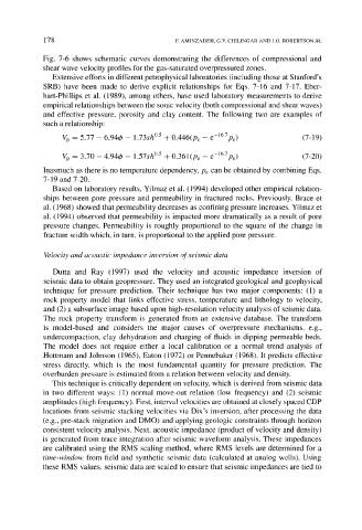
Fig. 7-6 shows schematic curves demonstrating the differences of compressional and
shear wave velocity profiles for the gas-saturated overpressured zones.
Extensive efforts in different petrophysical laboratories (including those at Stanford's
SRB) have been made to derive explicit relationships for Eqs. 7-16 and 7-17. Eber-
hart-Phillips et al. (1989), among others, have used laboratory measurements to derive
empirical relationships between the sonic velocity (both compressional and shear waves)
and effective pressure, porosity and clay content. The following two are examples of
such a relationship:

Vp -- 5.77 - 6.94q~ - 1.73sh ~ + 0.446(pe - e -167pe) (7-19)

Vp - 3.70 - 4.94~b - 1.57sh ~ + 0.361 (Pe - e-167pe) (7-20)
Inasmuch as there is no temperature dependency, Pe can be obtained by combining Eqs.
7-19 and 7-20.
Based on laboratory results, Yilmaz et al. (1994) developed other empirical relation-
ships between pore pressure and permeability in fractured rocks. Previously, Brace et
al. (1968) showed that permeability decreases as confining pressure increases. Yilmaz et
al. (1994) observed that permeability is impacted more dramatically as a result of pore
pressure changes. Permeability is roughly proportional to the square of the change in
fracture width which, in turn, is proportional to the applied pore pressure.

Velocity and acoustic impedance inversion of seismic data

Dutta and Ray (1997) used the velocity and acoustic impedance inversion of
seismic data to obtain geopressure. They used an integrated geological and geophysical
technique for pressure prediction. Their technique has two major components: (1) a
rock property model that links effective stress, temperature and lithology to velocity,
and (2) a subsurface image based upon high-resolution velocity analysis of seismic data.
The rock property transform is generated from an extensive database. The transform
is model-based and considers the major causes of overpressure mechanisms, e.g.,
undercompaction, clay dehydration and charging of fluids in dipping permeable beds.
The model does not require either a local calibration or a normal trend analysis of
Hottmam and Johnson (1965), Eaton (1972) or Pennebaker (1968). It predicts effective
stress directly, which is the most fundamental quantity for pressure prediction. The
overburden pressure is estimated from a relation between velocity and density.
This technique is critically dependent on velocity, which is derived from seismic data
in two different ways: (1) normal move-out relation (low frequency) and (2) seismic
amplitudes (high frequency). First, interval velocities are obtained at closely spaced CDP
locations from seismic stacking velocities via Dix's inversion, after processing the data
(e.g., pre-stack migration and DMO) and applying geologic constraints through horizon
consistent velocity analysis. Next, acoustic impedance (product of velocity and density)
is generated from trace integration after seismic waveform analysis. These impedances
are calibrated using the RMS scaling method, where RMS levels are determined for a
time-window from field and synthetic seismic data (calculated at analog wells). Using
these RMS values, seismic data are scaled to ensure that seismic impedances are tied to