Page 173 - Orlicky's Material Requirements Planning

152 PART 2 Concepts

2
cost is at the point where the inventory (carrying) cost and setup cost are equal.” This
holds true for the EOQ approach but not for the discrete lot-sizing approach, which
assumes that inventory depletions occur at the beginning of each period, as pointed out
previously.
In the graphic model of the general relationship between setup and carrying costs,
the total cost is at a minimum at the point of intersection of the carrying-cost line and the
setup curve only when the line passes through origin (point 0 on the X and Y axes). In
the discrete lot-sizing model, however, if a line were fitted to the carrying-cost points, it
would have a negative intercept, caused by the assumption that the quantity equal to the
demand in the first period incurs no carrying cost. This point can best be illustrated on a
model of a series of uniform discrete demands, such as
Period: 1 2 3 4 5 6 7
Demand 20 0 20 0 20 0 20
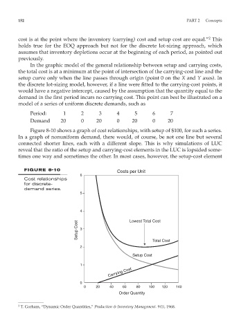
Figure 8-10 shows a graph of cost relationships, with setup of $100, for such a series.
In a graph of nonuniform demand, there would, of course, be not one line but several
connected shorter lines, each with a different slope. This is why simulations of LUC
reveal that the ratio of the setup and carrying-cost elements in the LUC is lopsided some-
times one way and sometimes the other. In most cases, however, the setup-cost element

FIGURE 8-10
Costs per Unit
6
Cost relationships
for discrete-
demand series.
5

4

Setup Cost 3 Lowest Total Cost

Total Cost
2
Setup Cost
1
Carrying Cost

0
0 20 40 60 80 100 120 140
Order Quantity

2 T. Gorham, “Dynamic Order Quantities,” Production & Inventory Management. 9(1), 1968.