Page 170 - Orlicky's Material Requirements Planning

CHAPTER 8 Lot Sizing 149

FIGURE 8-4
Period 1 2 3 4 5 6 7 8 9 Total
Fixed-period
requirements. New Requirements 35 10 40 20 5 10 30 150
Planned-Order Coverage 40 40 25 40 150

Period Order Quantity (POQ)

This technique, sometimes called economic time cycle, is based on the logic of the classic
EOQ modified for use in an environment of discrete period demand. Using known future
demand as represented by the net requirements schedule of a given inventory item, the
EOQ is computed through the standard formula to determine the number of orders per
year that should be placed. The number of planning periods constituting a year then is
divided by this quantity to determine the ordering interval. The POQ technique is iden-
tical to the one just discussed except that the ordering interval is computed.
Both these fixed-interval techniques avoid remnants in an effort to reduce inventory
carrying cost. For this reason, the POQ approach is more effective than the EOQ approach
because setup cost per year is the same but carrying cost will tend to be lower under
POQ. A potential difficulty with this approach, however, lies in the possibility that dis-
continuous net requirements will be distributed in such a way that the predetermined
ordering interval will prove inoperative. This will happen when several of the periods
coinciding with the ordering interval show zero requirements, thus forcing the POQ tech-
nique to order fewer times per year than intended.
Using the previous EOQ example and the annualized demand data, the POQ is
determined as follows:

EOQ 58
Number of periods in a year 12
Annual demand 200
250/58 3.4 (orders per year)
12/3.4 3.5 (ordering interval)

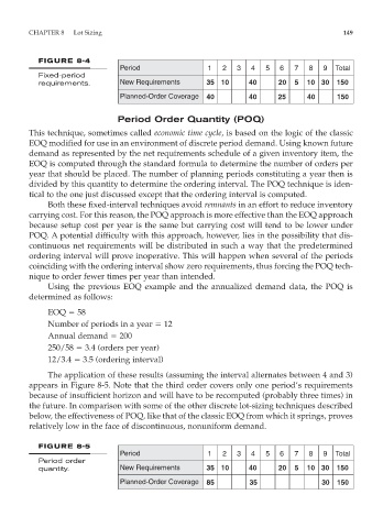
The application of these results (assuming the interval alternates between 4 and 3)
appears in Figure 8-5. Note that the third order covers only one period’s requirements
because of insufficient horizon and will have to be recomputed (probably three times) in
the future. In comparison with some of the other discrete lot-sizing techniques described
below, the effectiveness of POQ, like that of the classic EOQ from which it springs, proves
relatively low in the face of discontinuous, nonuniform demand.

FIGURE 8-5
Period 1 2 3 4 5 6 7 8 9 Total
Period order
quantity. New Requirements 35 10 40 20 5 10 30 150
Planned-Order Coverage 85 35 30 150