Page 169 - Orlicky's Material Requirements Planning

148 PART 2 Concepts

The EOQ is based on an assumption of continuous, steady-rate demand, and it will
perform well only where the actual demand approximates this assumption. In our exam-
ple, the demand is both discontinuous and nonuniform. The more discontinuous and
nonuniform the demand, the less effective the EOQ will prove to be.

Lot-for-Lot Ordering (L4L)

This technique, sometimes also referred to as discrete ordering, is the simplest and most
straightforward of all. It provides period-by-period coverage of net requirements, and the
planned-order quantity always equals the quantity of the net requirements being cov-
ered. These order quantities are, by necessity, dynamic; that is, they must be recomputed
whenever the respective net requirements change. Use of this technique minimizes
inventory carrying cost. It is often used for expensive purchased items and for any items,
purchased or manufactured, that have highly discontinuous demand. Conversely, items
in high-volume production and items that pass through specialized facilities geared to
continuous production (equivalent to permanent setup) normally are also ordered lot for
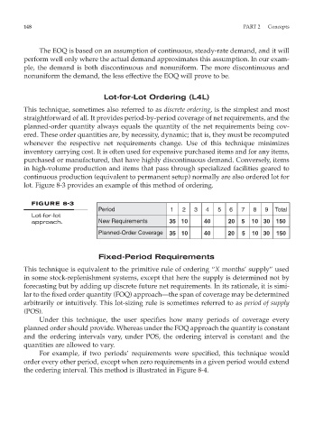
lot. Figure 8-3 provides an example of this method of ordering.

FIGURE 8-3
Period 1 2 3 4 5 6 7 8 9 Total
Lot-for-lot
approach. New Requirements 35 10 40 20 5 10 30 150
Planned-Order Coverage 35 10 40 20 5 10 30 150

Fixed-Period Requirements

This technique is equivalent to the primitive rule of ordering “X months’ supply” used
in some stock-replenishment systems, except that here the supply is determined not by
forecasting but by adding up discrete future net requirements. In its rationale, it is simi-
lar to the fixed order quantity (FOQ) approach—the span of coverage may be determined
arbitrarily or intuitively. This lot-sizing rule is sometimes referred to as period of supply
(POS).
Under this technique, the user specifies how many periods of coverage every
planned order should provide. Whereas under the FOQ approach the quantity is constant
and the ordering intervals vary, under POS, the ordering interval is constant and the
quantities are allowed to vary.
For example, if two periods’ requirements were specified, this technique would
order every other period, except when zero requirements in a given period would extend
the ordering interval. This method is illustrated in Figure 8-4.