Page 168 - Orlicky's Material Requirements Planning

CHAPTER 8 Lot Sizing 147

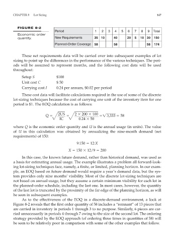
FIGURE 8-2
Period 1 2 3 4 5 6 7 8 9 Total
Economic order
quantity. New Requirements 35 10 40 20 5 10 30 150
Planned-Order Coverage 58 58 58 174

These net requirements data will be carried over into subsequent examples of lot
sizing to point up the differences in the performance of the various techniques. The peri-
ods will be assumed to represent months, and the following cost data will be used
throughout:
Setup S $100
Unit cost C $ 50
Carrying cost I 0.24 per annum, $0.02 per period
These cost data will facilitate calculations required in the use of some of the discrete
lot-sizing techniques because the cost of carrying one unit of the inventory item for one
period is $1. The EOQ calculation is as follows:

Q 2US 2 200 100 3,333 58
IC 0.24 50
where Q is the economic order quantity and U is the annual usage (in units). The value
of U in this calculation was obtained by annualizing the nine-month demand (net
requirements) of 150:

9:150 12:X
X 150 12/9 200

In this case, the known future demand, rather than historical demand, was used as
a basis for estimating annual usage. The example illustrates a problem all forward-look-
ing lot-sizing techniques face, namely, a finite, or limited, planning horizon. In our exam-
ple, an EOQ based on future demand would require a year’s demand data, but the sys-
tem provides only nine months’ visibility. Most of the discrete lot-sizing techniques are
not based on annual usage, but they assume a certain minimum visibility for each lot in
the planned-order schedule, including the last one. In most cases, however, the quantity
of the last lot is truncated by the proximity of the far edge of the planning horizon, as will
be seen in subsequent examples.
As to the effectiveness of the EOQ in a discrete-demand environment, a look at
Figure 8-2 reveals that the first order quantity of 58 includes a “remnant” of 13 pieces that
are carried in inventory in periods 1 through 3 to no purpose. Similarly, 6 pieces are car-
ried unnecessarily in periods 4 through 7 owing to the size of the second lot. The ordering
strategy provided by the EOQ approach (of ordering three times in quantities of 58) will
be seen to be relatively poor in comparison with some of the other examples that follow.