Page 171 - Orlicky's Material Requirements Planning

150 PART 2 Concepts

Least Unit Cost (LUC)

This technique and the three that follow have certain things in common. All of them
allow both the lot size and the ordering interval to vary. They share a common assump-
tion of discrete inventory depletions at the beginning of each period, which means that a
portion of each order, equal to the quantity of net requirements in the first period covered
by the order, is consumed immediately on arrival in stock and thus incurs no inventory
carrying charge. Inventory carrying cost, under all four of these lot-sizing methods, is
computed on the basis of this assumption rather than on average inventories in each peri-
od. All four of the techniques share the EOQ objective of minimizing the sum of setup
and inventory carrying costs, but each of them employs a somewhat different attack.
The LUC technique is best explained in terms of trial and error, and this approach is
used here, although less primitive methods of computation do exist. In determining the
order quantity, the LUC technique asks, in effect, whether this quantity should equal the
first period’s net requirements or should be increased to cover the next period’s require-
ments or the one after that, and so on. The decision is based on the unit cost (i.e., setup plus
inventory carrying cost per unit) computed for each of the successive order quantities. The
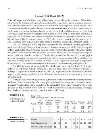
one with the least unit cost is chosen to be the lot size. Figure 8-6 shows the computation
of the first lot. The next one is computed in identical fashion starting with period 4.
The LUC is found at lot quantity 45, which will cover periods 1 and 2. The next
order of 60 will cover periods 4 through 6, and the third order of 45 will cover periods 7
through 9 (Figure 8-7). The limitation of the LUC approach lies in the fact that the tech-
nique considers only one lot at a time. The unit cost varies, sometimes widely, from one
lot to the next.
Tradeoffs between consecutive lots sometimes could be made that would reduce the
total cost of two or more lots. Our example contains such a situation: If the requirement
in period 7 were added to the quantity of the second lot, its inventory carrying cost would
increase by $15, but that of the next lot would decrease by $40. The lot-sizing technique
described next attempts to overcome this flaw in LUC logic.

FIGURE 8-6
Setup: $100
Inventory carrying cost: $1 per unit per period
Computation of
least unit cost. Net Carried in Prospec- Carry cost, $
require- inventory tive lot Setup per Unit
Period ments (periods) size For lot Per unit unit, $ cost, $
1 35 0 35 0.00 0 2.86 2.86
2 10 1 45 10.00 .22 2.22 2.44
3 0 2 0
4 40 3 85 130.00 1.53 1.18 2.71

FIGURE 8-7
Period 1 2 3 4 5 6 7 8 9 Total
Least unit cost.
New Requirements 35 10 40 20 5 10 30 150
Planned-Order Coverage 45 60 45 150