Page 270 - PVT Property Correlations

236 PVT Property Correlations

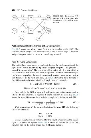
0.12 0.4 FIGURE 10.7 The example ANN
0.03 H1 0.01 structure with weight values after
0.15 0.2
initialization. ANN, artificial neural
network.
0.2
0.55
0.2 H2 0.99
0.4 0.55

0.3 0.7

Artificial Neural Network Initialization Calculations
Fig. 10.7 shows the initial values for the eight weights in the ANN. The
selection of the weights can be arbitrary or follow a certain logic. The initial
weights assigned to this network were randomly selected.

Feed-Forward Calculations
The hidden layer node values are calculated using the total summation of the
input node values multiplied by their assigned weights. This process is
termed “transformation.” The bias node with a weight of 1.0 is also added to
the summation. The use of bias nodes is optional. Note that other techniques
can be used to perform the transformation calculations; however, the weight
sum technique is the most common. Eq. (10.1) shows the basic formula of
the hidden node value determination through the total summation.
H1 5 W1 3 I1 1 W2 3 I2 1 B1 3 1 ð10:1Þ
H1 5 0:12 3 0:03 1 0:15 3 0:2 1 0:3 3 1 5 0:334

Each node in the hidden layer will undergo the activation function calcu-
lations. In this example, a sigmoid S-shape function is used. Eq. (10.2)
shows the sigmoid function form and the example calculation for node H1.
1 1
H1out 5 5 5 0:583 ð10:2Þ
1 1 e 2H1 1 1 e 20:334
With completion of the same calculations for node H2, the following
values are obtained:
H2 5 0:386
H2out 5 0:595
Similar calculations are performed for the output layers (using the hidden
layer node values as inputs). Table 10.4 summarizes the results of the first
iteration step for the output nodes (i.e., hidden and output).