Page 64 - Petrology of Sedimentary Rocks

that, unless the two properties are almost perfectly correlated, two trends lines can be
computed; let’s say we have a graph of feldspar content versus roundness, with a
correlation coefficient of +.45 (good, but far from perfect correlation). We can either
(I) compute the line to predict most accurately the roundness, given the feldspar
content; or (2) a line to predict most accurately the feldspar contents given the
roundness. The two lines may easily form a cross with as much as 30” or more
difference in angle. Again, these work only for straight-line trends; non-linear trends
require more complicated arithmetic.

To the trend line is usually attached a “standard error of estimate” band,
essentially equal to the standard deviation. This band runs parallel to the computed
trend and includes two-thirds of all the points in the scatter diagram. Its purpose is to
show the accuracy of the relationship. For example, in a certain brachiopod the length
and width of the shell are related by the equation L = 2W -I + 0.5. The last figure is
the standard error of estimate; if a given specimen has a width of 3.5 cm, the length is
most likely 8 cm, but we can expect two-thirds of the specimens to range between 7.5
and 8.5 cm. (one-sixth of them will be over 8.5 cm, and one-sixth under 7.5cm).

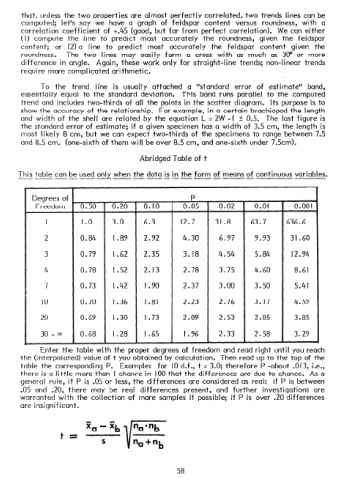
Abridged Table of t

This table can be used only when the data is in the form of means of continuous variables.
-----
-__--------
Degrees of
Freedom 0.50 0.20 0. IO 0.02 0.01 0.001

I 1.0 3.0 6.3 12.7 31.8 63.7 636.6

2 0.84 1.89 2.92 4.30 6.97 9.93 31.60

3 0.79 1.62 2.35 3. I8 4.54 5.84 12.94

4 0.78 I .52 2. I3 2.78 3.75 4.60 8.61

7 0.73 I .42 I -. 90 2.37 3.00 3.50 5.41

IO 0.70 1.36 I .8l 2.23 2.76 3.17 4.59

20 0.69 1.30 1.73 2.09 2.53 2.85 3.85

30 - m 0.68 1.28 1.65 I .96 2.33 2.58 3.29

Enter the table with the proper degrees of freedom and read right until you reach
the (interpolated) value of t you obtained by calculation. Then read up to the top of the
table the corresponding P. Example: for IO d.f., t = 3.0; therefore P -about .013, i.e.,
there is a little more than I chance in 100 that the differences are due to chance. As a
general rule, if P is .05 or less, the differences are considered as real: if P is between
.05 and .20, there may be real differences present, and further investigations are
warranted with the collection of more samples if possible; if P is over .20 differences
are insignificant.
xa -x’
b
t =
S

58