Page 62 - Petrology of Sedimentary Rocks

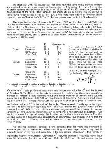
We start out with the assumption that both have the same heavy mineral content
and proceed to compute our expected frequencies on this basis. To figure the number
of green tourmalines expected in a count of 45 grains of the Eli formation, we decide
(from looking at the totals) that 40/96 of the grains should be green; thus we expect 45
times 40/96 green grains in the Eli, or 18.7. Since there were a total of 40 green grains
counted, then we’d expect 40-18.7 or 21.3 green grains to occur in the Nineteenten.

The expected number of browns is 45 times 22/96 or 10.3 for Eli, and 22-10.3 or
I 1.7 for Nineteenten. For “others” we expect 45 times 34/96 or 15.9 for Eli, and 34-
15.9 or 18.1 for Nineteenten. Now we set up the following table, subtracting 0.5 from
each of the differences, giving our corrected differences (the reason we subtract 0.5
from each difference is a “correction for continuity” because obviously you cannot
count fractional grains, and IO grains is as close as you can possibly get to an expected
frequency of 10.3 grains).

Eli Nineteenten
Observed I5 25 For each of the six “cells”
Green Expected 18.7 21.3 (three tourml’aline varieties in
Difference 3.7 3.7 each of two formations) we
Corr. Diff. 3.2 3.2 square the corrected differ-
ence and divide it by the ex-
for’ that
Observed IO I2 pected frequency --- one
Brown Expected 10.3 II.7 cell. Then we add UD these
Difference 0.3 0.3 values for the entire six cells
Corr. Diff. 0.3 0 and the total gives us the val-
ue of X2 , in this example 2.56.
Observed 20 I4 ,I .I. *. .
Other Expected 15.9 18. I Symbolicarry, tnrs operarron IS
Difference 4. I 4. I
Corr. Diff. 3.6 3.6 X2 II

0
x2 = -+-+-+ 10.24 0 -+-++$= 12.95 2.56
10.24
18.7 21.3 10.3 11.7 5.9
We enter a X2 table (p. 60) and must know two things: our value for X2 and the degrees
of freedom (d.f.). This time the d.f. is obtained by multiplying these two quantities:
(number of horizontal data columns minus one) times (number of vertical data columns
minus one); in this case (3-l X2-I), or two degrees of freedom. Again, we read across
the horizontal row corresponding with the proper number of degrees of freedom until

we find our value of X2 in the body of the table. Then we read directly up to the top of
the table to find the corresponding “P”. This will answer the question, what are the
chances (out of 100) that such differences--or larger--would be obtained in random
sampling of two uniform formations (or in sampling a homogeneous population?) Our
result came out P = approximately .20, in other words there is one chance in five that
we have sampled a homogeneous population, or conversely, four chances in five that the
formations have a differing tourmaline content-- though this last statement is not
strictly true.

For another example, consider a tire company that for years has averaged 31
blowouts per million tire miles. After switching to a new type rubber, they find 44
blowouts occur in the next million miles. Is the new rubber inferior, or is this merely an

expectable chance fluctuation ? Using the X2 test, the expected frequency would have
been 31 blowouts for the new tires. (O-E) is 44-31 or 13, and correcting for

56