Page 58 - Petrology of Sedimentary Rocks

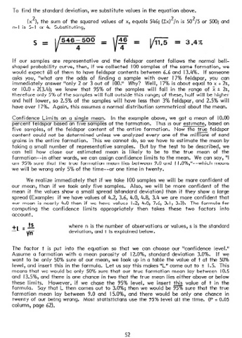
To find the standard deviation, we substitute values in the equation above.

(x2), the sum of the squared values of x, equals 546; (Cx)2/n is 502/5 or 500; and
n-l is 5-l or 4. Substituting,
s = /y= = F = /-iiz = 3.4%

If our samples are representative and the feldspar content follows the normal bell-
shaped probability curve, then, if we collected 100 samples of the same formation, we
would expect 68 of them to have feldspar contents between 6.6 and 13.4%. If someone
asks you, “what are the odds of finding a sample with over 17% feldspar, you can
immediately answer “only 2 or 3 out of 100.” Why? Well, 17% is about equal to x + 2s,
or 10.0 + 2t3.4); we know that 95% of the samples will fall in the range of X 2 2s,
therefore only 5% of the samples will fall outside this range; of these, half will be higher
and half lower, so 2.5% of the samples will have less than 3% feldspar, and 2.5% will
have over 17%. Again, this assumes a normal distribution symmetrical about the mean.

Confidence Limits on a single mean. In the example above, we got a mean of 10.00
percent feldspar based on five samples of the formation. This is our estimate, based on
five samples, of the feldspar content of the entire formation. Now the true feldspar
content could not be determined unless we analyzed every one of the millions of sand
grains in the entire formation. This we cannot do, so we have to estimate the mean by
taking a small number of representative samples. But by the test to be described, we
can tell how close our estimated mean is likely to be to the true mean of the
formation--in other words, we can assign confidence limits to the mean. We can say, “I
am 95% sure that the true formation mean lies between 9.0 and I I.O%,“--which means
we will be wrong only 5% of the time--or one time in twenty.

We realize immediately that if we take 100 samples we will be more confident of
our mean, than if we took only five samples. Also, we will be more confident of the
mean if the values show a small spread (standard deviation) than if they show a large
spread (Example: if we have values of 4.2, 3.6, 4.0, 4.8, 3.4 we are more confident that
our mean is nearly 4.0 than if we have values 1.2, 4.8, 7.6, 3. I, 3.3). The formula for
computing the confidence limits appropriately then takes these two factors into
account.

where n is the number of observations or values, s is the standard
deviation, and t is explained below.

The factor t is put into the equation so that we can choose our “confidence level.”
Assume a formation with a mean porosity of 12.0%, standard deviation 3.0%. If we
want to be only 50% sure of our mean, we look up in a table the value of t at the 50%
level, and insert this in the formula. Let us say this makes “L” come out to + 1.5. This
means that we would be only 50% sure that our true formation mean lay between 10.5
and 13.5%, and there is one chance in two that the true mean lies either above or below
these limits. However, if we chose the 95% level, we insert this value of t in the
formula. Say that L then comes out to 3.0%; then we would be m sure that the true
formation mean lay between 9.0 and 15.0%, and there would be only one chance in
twenty of our being wrong. Most statisticians use the 95% level all the time. (P = 0.05
column, page 62).

52