Page 198 - Petrophysics 2E

PERMEABILITY-POROSITY RELATIONSHIPS 171

TABLE 3.8
INTERMEDIATE CALCULATING VARIANCE FOR WELL HBK5
RESULTS
FOR
Interval k, mD In (ki) n(ln kl In kz ... ln k14) C(ki - k)2
1 120 4.7875 4.7875E+00 0.0781
2 213 5.3613 2,5667E+0 1 0.1647
3 180 5.1930 1.3329E+O2 0.1806
4 200 5.2983 7.0620E+02 0.2342
5 212 5.3566 3.7828E+03 0.3181
6 165 5.1059 1.93 15E+04 0.3196
7 145 4.9767 9.6126E+04 0.3278
8 198 5.2883 5.0834E+05 0.3768
9 210 5.3471 2.7 181 E+O6 0.4553
10 143 4.9628 1.3490E+07 0.4661
11 79 4.3694 5.8942E+07 0.9525
12 118 4.7707 2.8 120E+08 1.0403
13 212 5.3566 1.5063E+09 1.1242
14 117 4.7622 7.1730E+09 1.2171

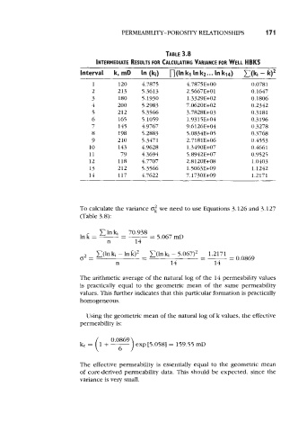
To calculate the variance $ we need to use Equations 3.126 and 3.127
(Table 3.8):

- Clnki 70.938
Ink=-=-- n 14 - 5.067 mD

---
2 C(lnki - C(lnki - 5.067)2 - 1.2171
-
o= - - 0.0869
n 14 14
The arithmetic average of the natural log of the 14 permeability values
is practically equal to the geometric mean of the same permeability
values. This further indicates that this particular formation is practically
homogeneous.

Using the geometric mean of the natural log of k values, the effective
permeability is:

ke = (1 + 7) exp[5.058] = 159.55 mD

The effective permeability is essentially equal to the geometric mean
of corederived permeability data. This should be expected, since the
variance is very small.