Page 199 - Petrophysics 2E

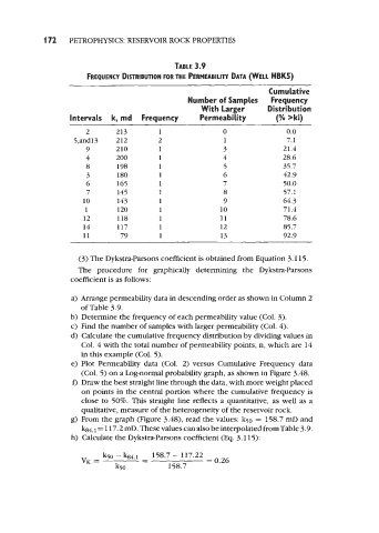
172 PETROPHYSICS: RESERVOIR ROCK PROPERTIES

TABLE 3.9
FREQUENCY DISTRIBUTION FOR THE PERMEABILITY DATA WELL HBK5)

Cumulative
Number of Samples Frequency
With Larger Distribution
Intervals k, md Frequency Permeability ("YO >ki)

2 213 1 0 0.0
5,and13 212 2 1 7.1
9 210 1 3 21.4
4 200 1 4 28.6
8 198 1 5 35.7
3 180 1 6 42.9
6 165 1 7 50.0
7 145 1 8 57.1
10 143 1 9 64.3
1 120 1 10 71.4
12 118 1 11 78.6
14 117 1 12 85.7
11 79 1 13 92.9

(3) The Dykstra-Parsons coefficient is obtained from Equation 3.1 15.
The procedure for graphically determining the Dykstra-Parsons
coefficient is as follows:

Arrange permeability data in descending order as shown in Column 2
of Table 3.9.
Determine the frequency of each permeability value (Col. 3).
Find the number of samples with larger permeability (Col. 4).
Calculate the cumulative frequency distribution by dividing values in
Col. 4 with the total number of permeability points, n, which are 14
in this example (Col. 5).
Plot Permeability data (Col. 2) versus Cumulative Frequency data
(Col. 5) on a Log-normal probability graph, as shown in Figure 3.48.
Draw the best straight line through the data, with more weight placed
on points in the central portion where the cumulative frequency is
close to 50%. This straight line reflects a quantitative, as well as a
qualitative, measure of the heterogeneity of the reservoir rock.
From the graph (Figure 3.48), read the values: k5o = 158.7 mD and
117.2 rnD. These values can also be interpolated from Table 3.9.
Calculate the Dykstra-Parsons coefficient (Eq. 3.1 15):

k50 - b4.1 - 158.7 - 117.22
VK = - = 0.26
k50 158.7