Page 308 - Petrophysics 2E

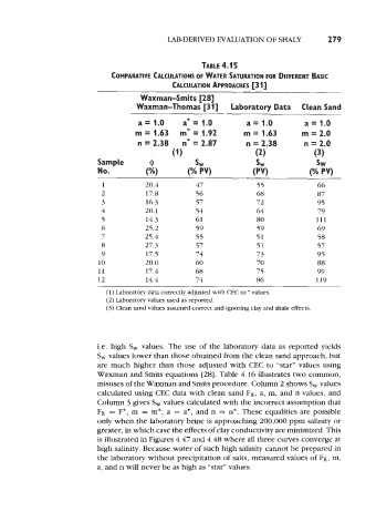
LABDERIVED EVALUATION OF SHALY 279

TABLE 4.1 5
COMPARATIVE CALCULATIONS OF WATER SATURATION FOR DIFFERENT BASIC
CALCUIATION APPROACHES [3 13
Waxman-Smits [28]
Waxman-Thomas [3 11 Laboratory Data Clean Sand

a= 1.0 a* = 1.0 a= 1.0 a= 1.0
m = 1.63 m* = 1.92 m = 1.63 m = 2.0
n = 2.38 n* = 2.87 n = 2.38 n = 2.0
(1) (2) (3)
Sample @ SW SW SW
No. (%I (% PV) (PV) (% PV)

1 20.4 47 55 66
2 17.8 56 68 87
3 16.3 57 72 95
4 20.1 54 64 79
5 14.3 61 80 111
6 25.2 59 59 69
7 25.4 55 51 58
8 27.3 57 51 57
9 17.5 74 73 95
10 20.0 60 70 88
11 17.4 68 75 99
12 14.4 74 86 119
~~ ~ ~
(1) Laboratory data correctly adjusted with CEC to * values.
(2) Laboratory values used as reported.
(3) Clean sand values assumed correct and ignoring clay and shale effects.

i.e. high S, values. The use of the laboratory data as reported yields
S, values lower than those obtained from the clean sand approach, but
are much higher than those adjusted with CEC to “star” values using
Waxman and Smits equations [28]. Table 4.16 illustrates two common,
misuses of the Waxman and Smits procedure. Column 2 shows S, values
calculated using CEC data with clean sand FR, a, m, and n values, and
Column 3 gives S, values calculated with the incorrect assumption that
FR = F*, m = m*, a = a*, and n = n*. These equalities are possible
only when the laboratory brine is approaching 200,000 ppm salinity or
greater, in which case the effects of clay conductivity are minimized. This
is illustrated in Figures 4.47 and 4.48 where all three curves converge at
high salinity. Because water of such high salinity cannot be prepared in
the laboratory without precipitation of salts, measured values of FR, m,
a, and n will never be as high as “star” values.