Page 155 - Phase Space Optics Fundamentals and Applications

136 Chapter Four

3 2 3 2
Spatial coordinate (mm) –1 1 0 Spatial coordinate (mm) –1 1 0

–2
–3
–3 –2
0 15 30 45 60 75 90 0 15 30 45 60 75 90
Projection angle (°) Projection angle (°)
(a) (b)

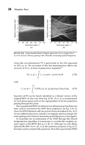
FIGURE 4.16 Experimental Radon-Wigner spectrum of (a) a single slit of
2.2 mm and (b) a binary grating with a linearly increasing spatial frequency.

where the one-dimensional FT is performed on the first argument
of RW f (x , ). The inversion of this last transformation allows the
recovery of W f (x, ) from its projections. Explicitly 34

W f (x, ) = C f (x cos + sin , ) d (4.78)
0
with
+∞

C f (u, ) = F{RW f (x , ), } | | exp (i2 u) d (4.79)
−∞
Equation (4.79) can be clearly identified as a filtered version of the
original RWT. In this way, from Eq. (4.78), W f (x, ) is reconstructed
for each phase-space point as the superposition of all the projections
passing through this point.
The experimental RWD of different one-dimensional functions has
been used to reconstruct the WDF from projections. In Fig. 4.16 we
show the RWD obtained with the optical device described in Sec. 4.2.2
for two different functions, namely, a rectangular aperture (single slit)
andagratingwithalinearlyincreasingspatialfrequency(chirp signal).
To undertake the reconstruction of the WDF through the filtered
backprojection algorithm, it is necessary to consider the complete an-
gular region of the RWD, that is, ∈ [0, ). Although we only obtain
optically the RWT for ∈ [0, /2], the symmetry property in Eq. (4.17)
has been used to complete the spectrum. From the experimental RWD