Page 237 - Photodetection and Measurement - Maximizing Performance in Optical Systems

Measurand Modulation

230 Chapter Ten

1/Year 1/month
Noise Density (Arb.) 1/hour 1Hz 1kHz

Frequency

1.6
1.4
Signal Voltage 0.8 In Operation
1.2
1

0.6
0.4
0.2 Calibration
0
0 100 200 300 400 500 600 700 800 900 1000
Time from Calibration (Sample No.)
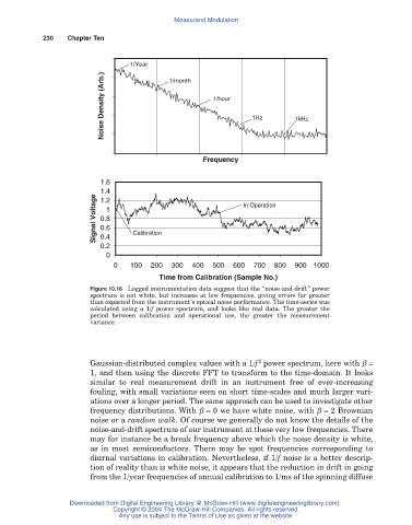
Figure 10.16 Logged instrumentation data suggest that the “noise-and-drift” power
spectrum is not white, but increases at low frequencies, giving errors far greater
than expected from the instrument’s optical noise performance. The time-series was
calculated using a 1/f power spectrum, and looks like real data. The greater the
period between calibration and operational use, the greater the measurement
variance.

b
Gaussian-distributed complex values with a 1/f power spectrum, here with b =
1, and then using the discrete FFT to transform to the time-domain. It looks
similar to real measurement drift in an instrument free of ever-increasing
fouling, with small variations seen on short time-scales and much larger vari-
ations over a longer period. The same approach can be used to investigate other
frequency distributions. With b = 0 we have white noise, with b = 2 Brownian
noise or a random walk. Of course we generally do not know the details of the
noise-and-drift spectrum of our instrument at these very low frequencies. There
may for instance be a break frequency above which the noise density is white,
as in most semiconductors. There may be spot frequencies corresponding to
diurnal variations in calibration. Nevertheless, if 1/f noise is a better descrip-
tion of reality than is white noise, it appears that the reduction in drift in going
from the 1/year frequencies of annual calibration to 1/ms of the spinning diffuse

Downloaded from Digital Engineering Library @ McGraw-Hill (www.digitalengineeringlibrary.com)
Copyright © 2004 The McGraw-Hill Companies. All rights reserved.
Any use is subject to the Terms of Use as given at the website.