Page 164 - Physical Principles of Sedimentary Basin Analysis

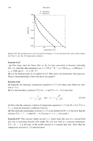
146 Heat flow

simulation
analytical
250

0

depth [m] −250

−500

−750
0 10 20 30
temperature [°C]
Figure 6.20. The geotherms for cases (a) and (b) in Figure 6.19 are shown for the center of the island.
See Note 6.4 for the 1D temperature solution.

Exercise 6.15
(a) How large must the Darcy flux v D be for heat convection to become noticeable
(Pe = 1), when the other parameters are λ = 2W m −1 K −1 , l 0 = 300 m, f = 1000 kg m −3 ,
c f = 1000 and T 2 − T 1 = 50 C?
◦
(b) Let the fluid pressure in an aquifer be 0.5 MPa above the hydrostatic fluid pressure.
What is the permeability of the rock above the aquifer?

Exercise 6.16
(a) Integrate the stationary temperature equation (6.152) two times and obtain the solu-
tion (6.153).
ˆ
(b) Use the boundary conditions T (ˆz=0) = 1 and T (ˆz=1) = 0 to show that
ˆ
1 e Pe
c 1 = and c 2 =− . (6.164)
1 − e Pe 1 − e Pe

ˆ
(c) Show that the stationary solution of temperature equation (6.152) for Pe = 0is T (ˆz) =
1 −ˆz, using the boundary conditions from (b).
(d) The stationary temperature solution (6.154) is not defined for Pe = 0, but show that the
x
solution T (ˆz) → 1 −ˆz when Pe → 0. Use that e ≈ 1 + x for small x.
ˆ
Exercise 6.17 This exercise builds on note 6.4, which treats the case of a vertical fluid
flux that is increasing linearly with depth. We will now look at a constant temperature
ˆ
T (ˆz = 0) = 1 at the base of the model instead of a constant heat flux. Show that the
temperature solution (6.158) then becomes