Page 196 - Physical Principles of Sedimentary Basin Analysis

178 Heat flow

50 0
observations observations
50
100 linear fit
100
150
depth [m] depth [m] 150 step
200
200
periodic linear increase
250
250

300 300
6.5 7.0 7.5 8.0 8.5 9.0 −0.5 0.0 0.5 1.0 1.5
temperature [°C] temperature difference [°C]
(a) (b)
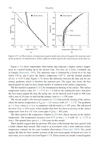
Figure 6.37. (a) Observations of temperature against depth and a linear fit against the stationary part
of the geotherm. (b) Optimization of three different models against the transient part of the data set.

Figure 6.37a shows temperature observations that indicates a higher surface temper-
ature in a period leading up to the present time. The data set is from a borehole site
in Canada (Mareschal, 2005). The stationary state is obtained by a linear fit of the data
◦
below 170 m, and it gives the surface temperature 6.07 C, and the thermal gradient
◦
dT/dz = 9.15 C/km. Figure 6.37b shows the difference between the data and the sta-
tionary geotherm, which is therefore the transient part. The figure also shows the best
match against the data for three simple models of variation in the surface temperature.
The first model is equation (6.202) for instantaneous heating of the surface. The surface
temperature makes a step T = 1.3 Cat t = 0 and we are seeking the time t that gives
◦
the best match against the data. By trying out t in the interval from 0 years to 500 years
with a step of 10 years we find that the optimal value is t 1 = 150 years.
The second model is the thermal transient (6.273) from periodic heating of the surface,
where the surface temperature is T surf (t) = T cos(ωt) with T = 1.3 C. The geotherm
◦
at t = 2πt 0 , where t 0 = 1/ω, is optimized with the result t 0 = 257 years. The full period
becomes 2πt 0 = 1614 years, which implies that there has been an increase in the surface
1
temperature from 0 to T over a time span of πt 0 = 403 years.
2
The third model is the temperature solution (6.283) for a linear increase in the surface
temperature. The temperature increases from 0 C at time t = 0 until T = 1.3 Cat
◦
◦
time t. The optimal time span is t = 340 years for this model.
These models suggest that the previous 400 years at the boresite has had a period with
a hotter climate than normal. This result is in accordance with a more elaborate surface
temperature estimate for the same borehole observations (Mareschal, 2005). The match
against the data for these models in terms of the root-mean-square deviation are close to
each other, as we can also see from Figure 6.37b. These models are simple to match against