Page 255 - Physical Principles of Sedimentary Basin Analysis

7.12 Lithospheric extension and decompression melting 237

1150 C 1200 C 1250 C 1300 C
0

50 liquidus
depth [km] 100 X=25% X=75%

X=50%

150

200 solidus
1000 1250 1500 1750 2000
temperature [°C]
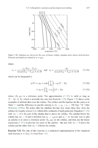
Figure 7.26. Adiabats are shown for the case of linear solidus, liquidus and a linear melt fraction.
Pressure and depth are related by p = gz.

where
c p (T l,0 − T s,0 ) s
a 1 = and a 2 = (7.151)
(α/ )(T l,0 − T s,0 ) + sB (α/ )(T l,0 − T s,0 ) + sB
which can be integrated to

T
p(T ) = p 0 + a 1 ln + a 2 (T − T 0 ) (7.152)
T 0

a 1
≈ p 0 + + a 2 (T − T 0 ) (7.153)
T 0
where (T 0 , p 0 ) is a reference point. The approximation (7.153) is valid as long as
|T − T 0 |
T 0 , which is normally the case (see Exercise 7.25). Figure 7.26 shows some
examples of adiabats that cross the solidus. The solidus and the liquidus are the same as in
Table 7.1 and the difference in specific entropy is s = s m − s s = 356 J kg −1 K −1 after
McKenzie (1984). We notice that the adiabats become less steep when they cross the
solidus, by roughly a factor 1/2, which affect estimates of melt generated. Equation (7.152)
with s > 0 is the part of the adiabat that is above the solidus. The adiabat below the
solidus has s = 0 and it therefore has a 1 = c p /α and a 2 = 0. An easy way to plot
an adiabat is to select a reference point (T 0 , p 0 ) on the solidus, and then use the linear
expression (7.153) to plot the two parts of the adiabat – the one with s > 0 above the
solidus and the other with s = 0 below the solidus.

Exercise 7.24 The aim of this exercise is a numerical implementation of the empirical
melt fraction X = X(p, T ) from Note 7.10.