Page 315 - Physical Principles of Sedimentary Basin Analysis
P. 315

9.4 Flexure and lateral variations of the load    297

                1.0                                  800

                0.8
                                                     600
                0.6
              c [−]                               λ c  [km]  400
                0.4

                                                     200
                0.2

                0.0                                    0
                  0     1    2    3    4    5           0   10    20   30   40   50
                             λ/λ  [−]                              h [km]
                               c
                               (a)                                  (b)
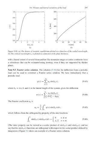
            Figure 9.10. (a) The degree of isostatic equilibrium plotted as a function of the scaled wavelength.
            (b) The critical wavelength λ c is plotted as a function of the plate thickness.

            with a lateral extent of several thousand km like mountain ranges or entire continents have
            a subsidence that can be estimated using isostasy, even if they are supported by thicker
            plates.
            Note 9.5 Fourier series solution. The solution (9.58) for the deflection from a periodic
            load can be used to construct a Fourier series solution. We have immediately that a
            periodic load
                                             ∞

                                      q(x) =    a n sin(k n x),                (9.63)
                                            n=1
            where k n = πn/L and L is the lateral length of the system, gives the deflection

                                             ∞
                                                a n sin(k n x)
                                     w(x) =               .                    (9.64)
                                                  4
                                               Dk +   g
                                            n=1   n
            The Fourier coefficient a n is
                                         2     L
                                    a n =     q(x) sin(k n x)dx,               (9.65)
                                         L  0
            which follows from the orthogonality property of the sine functions

                                L
                                                      0    n  = m
                                 sin(k n x) sin(k m x)dx =                     (9.66)
                              0                       L/2 n = m.
            (The latter property can be viewed as a scalar product of sin(k n x) and sin(k m x), and we
            saythatthesin(k n x)-functions are orthogonal with respect to the scalar product defined by
            integration.) Figure 9.8 shows an example of a Fourier series solution.
   310   311   312   313   314   315   316   317   318   319   320