Page 276 - Physical Chemistry

lev38627_ch08.qxd 3/14/08 12:54 PM Page 257

257
Industrial processes often involve gases at pressures of hundreds of atmospheres, so Section 8.9
chemical engineers are keenly interested in differences between real-gas and ideal-gas Taylor Series
properties. For a full discussion of such differences (which are called residual func-
id
tions or departure functions), see Poling, Prausnitz, and O’Connell, chap. 6. (S – S )/(cal/mol-K)
m
m
id
Let H (T, P) H (T, P) be the difference between ideal- and real-gas molar en-
m
m
thalpies at T and P. Unsuperscripted thermodynamic properties refer to the real gas.
id
P
Equations (5.16) and (5.30) give H (T, P) H (T, P) [T( V / T) V ] dP
m
m
P
m
0
m
P
id
and S (T, P) S (T, P) [( V / T) R/P ] dP , where the integrals are at con-
0
m
m
P
m
stant T and the prime was added to the integration variable to avoid using the symbol
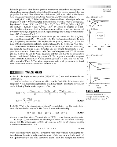
P with two meanings. Figures 8.11 and 8.12 plot enthalpy and entropy departure func-
tions of CH (g) versus T and P.
4
4
If we have a reliable equation of state for the gas, we can use it to find ( V / T) P CH (g)
m
id
id
and V and thus evaluate H H and S S . The virial equation of state in the form
m
m
m
m
m
(8.5) is especially convenient for this purpose, since it gives V and ( V / T) as func-
m
m
P
tions of P, allowing the integrals to be easily evaluated. For the results, see Prob. 8.23.
Unfortunately, the Redlich–Kwong and van der Waals equations are cubics in V m
and cannot be readily used in these formulas. One way around this difficulty is to ex-
pand these equations of state into a virial form involving powers of 1/V [for exam-
m
ple, Eq. (8.9) for the van der Waals equation] and then use (8.6) to put the equation id
m
into the virial form (8.5) involving powers of P. This approach is useful at low pres- (S – S )/(cal/mol-K)
m
sures. See Probs. 8.24 and 8.25. A more general approach is to use T and V as the vari-
ables, instead of T and P. This allows expressions valid at all pressures to be found
from the equation of state. For details, see Prob. 8.26.
8.9 TAYLOR SERIES
In Sec. 8.2, the Taylor series expansion (8.8) of 1/(1 x) was used. We now discuss
Taylor series.
Let f(x) be a function of the real variable x, and let f and all its derivatives exist at
the point x a and in some neighborhood of a. It may then be possible to express f(x)
as the following Taylor series in powers of (x a):
f¿1a21x a2 f–1a21x a2 2 f‡1a21x a2 3 Figure 8.12
f1x2 f1a2 p
1! 2! 3! Difference between real- and
ideal-gas molar entropy for CH 4
1n2
q f 1a2 plotted versus T and versus P.
n
f1x2 a 1x a2 (8.32)*
n 0 n!
(n)
n
n
In (8.32), f (a) is the nth derivative d f(x)/dx evaluated at x a. The zeroth deriv-
ative of f is defined to be f itself. The factorial function is defined by
n! n1n 121n 22 p # (8.33)*
2 1 and 0! 1
where n is a positive integer. The derivation of (8.32) is given in most calculus texts.
To use (8.32), we must know for what range of values of x the infinite series rep-
resents f(x). The infinite series in (8.32) will converge to f(x) for all values of x within
some interval centered at x a:
a c 6 x 6 a c (8.34)
where c is some positive number. The value of c can often be found by taking the dis-
tance between the point a and the real singularity of f(x) nearest to a. A singularity of
f is a point where f or one of its derivatives doesn’t exist. For example, the function